How to use pmlayer.torch.layers.PiecewiseLinear

In this tutorial, we demonstrate how to use pmlayer.torch.layers.PiecewiseLinear. The source code used in this tutorial is available at github.

The PiecewiseLinear layer transforms each dimension of the input features by using a piece-wise linear (PWL) function. You can construct a model that consists of a single PiecewiseLinear layer by using the following code.

import torch
from pmlayer.torch.layers import PiecewiseLinear

boundaries = torch.linspace(0.0, 1.0, 4)
model = PiecewiseLinear(boundaries, 2, indices_increasing=[0])

In this example, the endpoints of the PWL function is designated as the boundaries tensor. The constructor of PiecewiseLinear specifies that the size of input feature vector is 2, and the first input feature is designated as a monotonic feature by setting indices_increasing=[0]. This also means that we do not use the monotonicity constraint for the second input feature.

We can train this model to learn the function \(f(x) = 2(x-0.3)^2\) for each input by using the following code.

# prepare data
x = np.linspace(0.0, 1.0, 10)
y = 2.0*(x-0.3)*(x-0.3)
x = np.tile(x.reshape(-1,1), 2)
y = np.tile(y.reshape(-1,1), 2)
data_x = torch.from_numpy(x.astype(np.float32)).clone()
data_y = torch.from_numpy(y.astype(np.float32)).clone()

# train model
loss_function = nn.MSELoss()
optimizer = torch.optim.Adam(model.parameters(), lr=0.01)
for epoch in range(10000):
    pred_y = model(data_x)
    loss = loss_function(pred_y, data_y)
    loss.backward()
    optimizer.step()
    optimizer.zero_grad()

The results of the training can be verified by using the following code.

# plot
pred_y_np = pred_y.to('cpu').detach().numpy().copy()
fig = plt.figure(figsize=(7,3))
ax1 = plt.subplot(1, 2, 1)
ax2 = plt.subplot(1, 2, 2)

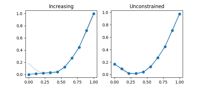
ax1.set_title('Increasing')
ax1.plot(x[:,0], y[:,0], color='gray', linestyle = 'dotted')
ax1.plot(x[:,0], pred_y_np[:,0], marker='o')
ax2.set_title('Unconstrained')
ax2.plot(x[:,1], y[:,1], color='gray', linestyle = 'dotted')
ax2.plot(x[:,1], pred_y_np[:,1], marker='o')
plt.show()

In the results, each blue solid line shows the learned function for an input feature and each dotted line shows the ground truth. Since the first input feature is designated as a monotonic feature, the neural network model is trained to learn the function under the constraint that the output is a monotonic function. In contrast, the second input feature is not designated as a monotonic feature, the neural network model is trained to learn the function without any constraints.