Solver algorithms¶

This chapter documents the timestep driver and acceptance logic of the stereographic dynamic integrator implemented in Z_sim_dynamic_stereo_base (demag and nodemag drivers). Configuration parameters are listed in Configuration reference.

Notation¶

The table lists symbols common to the timestep driver and to phases (A)–(C).

Symbol	Definition
\(t^n\), \(\Delta t^\ast\)	Physical time and non-dimensional timestep of the current attempt
\(\mathbf{u}^n=(\mathbf{q}_A^n,\mathbf{q}_B^n)\); demag adds \(\varphi^n\)	Accepted state at the beginning of the step (backup)
\(\mathbf{u}^{\mathrm{trial}}\)	State returned by the nonlinear solve prior to acceptance
\(\mathbf{F}(\mathbf{u})\)	\(\text{SNES}\) residual vector of the BDF-discretized LLG weak form (Stereographic formulation)
\(\\|\mathbf{F}\\|\)	Euclidean norm of the \(\text{SNES}\) residual vector
\(E_{\mathrm{split}}\), \(E_{\mathrm{phys}}\)	Split stored energy ((143)) and physical Cartesian energy ((145))
\(E_{\mathrm{gate}}\)	Energy functional monitored by the thermodynamic gate ((146))

Energy functionals¶

Each acceptance criterion in phases (C)–(F) compares a scalar energy or its increment step-over-step. The solver maintains two such scalars on every trial state: \(E_{\mathrm{split}}\) (compute_energy) and \(E_{\mathrm{phys}}`\) (_compute_energy_physical_cartesian). Both integrate the same micromagnetic energy densities over \(\Omega_{\mathrm{m}}\); they differ in how the magnetization field entering those densities is constructed from the dual-chart state \((\mathbf{q}_A,\mathbf{q}_B)\).

Split stored energy¶

\(E_{\mathrm{split}}\) is assembled directly from the stereographic chart fields. For each chart \(\chi\in\{A,B\}\), let \(\mathbf{m}_\chi = \mathbf{m}_\chi(\mathbf{q}_\chi)\) denote the Cartesian magnetization recovered from that chart’s inverse map, and let \(W_\chi\) denote the energy density evaluated on \(\mathbf{q}_\chi\) (for exchange, which uses stereographic gradients \(\nabla\mathbf{q}_\chi\)) or on \(\mathbf{m}_\chi\) (for anisotropy, Zeeman, and demagnetization). With element-wise atlas weights \(w_A\), \(w_B\),

(143)¶\[E_{\mathrm{split}} = \int_{\Omega_{\mathrm m}} \bigl(w_A\,W_A(\mathbf{q}_A) + w_B\,W_B(\mathbf{q}_B)\bigr) \,\mathrm{d}V^\ast = \mathcal{E}_{\mathrm{sol}}.\]

This is the functional whose Gateaux variation generates the \(\text{SNES}\) residual \(\mathbf{F}\) ((120), Stereographic formulation). Because exchange in \(W_\chi\) is expressed through stereographic gradients \(\nabla\mathbf{q}_\chi\) rather than \(\nabla\mathbf{m}\), \(E_{\mathrm{split}}\) depends on the full chart representation \((\mathbf{q}_A,\mathbf{q}_B)\) and not solely on the magnetization direction. compute_energy returns component integrals (exchange, uniaxial anisotropy, cubic anisotropy, demagnetization, Zeeman) followed by \(E_{\mathrm{split}}\).

Physical Cartesian energy¶

\(E_{\mathrm{phys}}\) evaluates the same energy densities on a single Cartesian field \(\mathbf{m}\) constructed by normalizing the atlas-weighted blend of the two chart reconstructions:

(144)¶\[\mathbf{m} = \frac{w_A\,\mathbf{m}_A(\mathbf{q}_A) + w_B\,\mathbf{m}_B(\mathbf{q}_B)} {|w_A\,\mathbf{m}_A + w_B\,\mathbf{m}_B| + \varepsilon}.\]

Exchange in \(E_{\mathrm{phys}}\) uses \(|\nabla\mathbf{m}|^2\) of this blended field; all other terms are evaluated identically to their counterparts in \(E_{\mathrm{split}}\). Formally,

(145)¶\[E_{\mathrm{phys}} = \int_{\Omega_{\mathrm m}} \Bigl( W_{\mathrm{ex}}(\mathbf{m}) + W_{\mathrm{ani}}(\mathbf{m}) + W_{\mathrm{d}}(\mathbf{m},\varphi) + W_{\mathrm{zee}}(\mathbf{m}) \Bigr)\,\mathrm{d}V^\ast,\]

computed by _compute_energy_physical_cartesian. Because \(\mathbf{m}\) is constructed from the blend without reference to individual chart gradients, \(E_{\mathrm{phys}}\) is a functional of the magnetization direction alone: it is insensitive to how the state \((\mathbf{q}_A,\mathbf{q}_B)\) is distributed between the two charts, provided the blended \(\mathbf{m}\) is the same.

Comparison and usage of the two functionals¶

When the two functionals agree. In regions where a single chart dominates, both charts reconstruct essentially the same magnetization direction, and the stereographic exchange gradient reduces to the physical one via the conformal factor. In that regime \(E_{\mathrm{split}}\) and \(E_{\mathrm{phys}}\) are numerically close.

When they differ. The two values are not equal in two situations. First, in overlap regions where both atlas weights are non-zero, each chart contributes independent stereographic gradients to \(E_{\mathrm{split}}\); those gradients do not need to match the gradient of the blended \(\mathbf{m}\) used by \(E_{\mathrm{phys}}\). Second, atlas closure (Atlas closure (phase F)) adjusts the chart fields \((\mathbf{q}_A,\mathbf{q}_B)\) to restore representation consistency without changing the physical magnetization, so \(E_{\mathrm{phys}}\) is unaffected while \(E_{\mathrm{split}}\) may shift.

Functional assignment by criterion. Each acceptance criterion uses exactly one of the two functionals:

Criterion	Functional	Rationale
\(\text{SNES}\) residual / \(F\)	\(E_{\mathrm{split}}\)	Gateaux derivative of (143).
Thermodynamic gate (\(E_{\mathrm{gate}}\), default)	\(E_{\mathrm{split}}\)	Form-consistent with the dynamical variables \(\mathbf{q}_{A,B}\) solved by \(\text{SNES}\).
Physical guard (optional, `thermo_enable_physical_guard`)	\(E_{\mathrm{phys}}\)	Secondary check that the blended-field energy has not grown; insensitive to chart redistribution inside the atlas.
Atlas closure jump	\(E_{\mathrm{gate}}\) (split or phys, per `thermo_use_split_energy`)	Monitors the energy change caused by the representational repair in phase (F); a large jump signals an inconsistent closure.
Steady-state stop	\(E_{\mathrm{phys}}\)	Atlas closure can shift \(E_{\mathrm{split}}\) without any physical change; \(E_{\mathrm{phys}}\) avoids spurious early termination near equilibrium.

Gate energy definition. The thermodynamic gate (phase E, Thermodynamic gate (phase E)) tests the increment \(\Delta E_{\mathrm{gate}} = E_{\mathrm{gate}}^{\mathrm{trial}} - E_{\mathrm{gate}}^{n}\) between the backup state \(\mathbf{u}^n\) and the trial state \(\mathbf{u}^{\mathrm{trial}}\). Flag thermo_use_split_energy (default True) selects which functional plays the role of \(E_{\mathrm{gate}}\). Let \(\chi\) denote that flag; then:

(146)¶\[\begin{split}E_{\mathrm{gate}} = \begin{cases} E_{\mathrm{split}} & \chi = \mathrm{True}, \\[0.4em] E_{\mathrm{phys}} & \chi = \mathrm{False}. \end{cases}\end{split}\]

Split stored energy (default, thermo_use_split_energy = True). The gate monitors \(E_{\mathrm{split}}\), the same functional whose Gateaux variation drives the \(\text{SNES}\) solve ((143), (120)). This keeps the energy test fully consistent with the dynamical degrees of freedom \((\mathbf{q}_A,\mathbf{q}_B)\) and with the functional differentiated in the nonlinear solve.
Physical Cartesian energy (thermo_use_split_energy = False). The gate monitors \(E_{\mathrm{phys}}\), which depends only on the blended magnetization \(\mathbf{m}\) ((145)). Because \(E_{\mathrm{phys}}\) is insensitive to how the state is distributed between charts, this option eliminates representational variation from the energy test. It is appropriate when the thermodynamic criterion must be stated strictly in terms of the physical magnetization direction rather than the atlas decomposition.

Structure of one timestep¶

At step index \(n\), solve_problem advances from the last accepted state \(\mathbf{u}^n\) at time \(t^n\) to an accepted state at \(t^{n+1}=t^n+\Delta t^\ast\). The routine nests several control levels; Figure 1 (Structure of one timestep) summarises the hierarchy.

Timestep loop. Outer driver for step in range(step_start, step_end) over integer indices \(n\). Physical time advances once per iteration, and only after a successful accept. Each iteration comprises three sequential blocks:

Preamble (_open_timestep, _run_timestep_preamble) — runs once before any retry at this \(n\). Updates demagnetization and Zeeman continuation ramps; when a ramp completes, transition guards may reduce \(\Delta t^\ast\), tighten growth caps, and rebase thermodynamic baselines (Continuation ramps).
Δt-retry loop (while not accepted) — repeated acceptance attempts at the current \(\Delta t^\ast\). The state \(\mathbf{u}^n\) is backed up before each attempt. If an attempt fails, the backup is restored and \(\Delta t^\ast\) may be reduced before retrying; the clock does not advance (Rejection and recovery). Each pass through this loop executes phases (A)–(F) on a trial state \(\mathbf{u}^{\mathrm{trial}}\) via _run_accept_attempt (Acceptance phases).
Post-acceptance update (_finalize_accepted_step) — runs once after accept. Advances \(t^n\to t^{n+1}\), updates BDF history, selects the next \(\Delta t^\ast\) ((176)), and writes I/O.

Operator-split loop (demag driver only). Inside phase (A) of a single acceptance attempt, a fixed-point iteration couples \(\text{SNES}\) for \((\mathbf{q}_A,\mathbf{q}_B,\varphi)\) with magnetostatic updates of \(\mathbf{H}_{\mathrm{d}}\) (Nonlinear solve (phase A)). This loop is nested within one acceptance attempt; it is not part of the timestep loop or the Δt-retry loop.

Acceptance phases¶

Within one iteration of the Δt-retry loop, the trial state passes through six phases (A)–(F) in order. Phases (A)–(E) operate on the dynamical chart fields; phase (F) repairs the stereographic representation for storage and I/O.

(A) Nonlinear solve (Nonlinear solve (phase A)). Advance the LLG equation over \([t^n,t^{n+1}]\) with a BDF formula on the chart variables \((\mathbf{q}_A,\mathbf{q}_B)\) (and \(\varphi\) in the demag driver), producing a trial state \(\mathbf{u}^{\mathrm{trial}}\) and a \(\text{SNES}\) residual \(F\). In the demag driver, magnetostatics and magnetization are coupled through an operator-split loop nested inside this phase.

(B) Algebraic validity (Algebraic validity (phase B)). Confirm that the nonlinear and linear algebra completed successfully: \(\text{SNES}\) and \(\text{KSP}\) converged, and in the demag driver the operator-split fixed point reached its tolerance. This phase does not evaluate physics; it only excludes diverged or incomplete solves.

(C) Atlas radius guard (Atlas guard (phase C)). Verify that the stereographic coordinates \(\mathbf{q}_A\), \(\mathbf{q}_B\) remain within a numerically safe range, and snapshot \(E_{\mathrm{split}}\) and \(E_{\mathrm{phys}}\) for the downstream gates. The energy snapshot is also refreshed whenever backtracking in phase (D) or (E) modifies the chart fields.

(D) Residual gate (Residual gate (phase D)). Compare \(\|\mathbf{F}\|\) against a history-adaptive threshold \(g_{\mathrm{res}}\). If the test fails, three substages are tried in order: residual backtracking along the chord between \(\mathbf{u}^n\) and \(\mathbf{u}^{\mathrm{trial}}\) (D1), merit acceptance based on the contraction of \(\|\mathbf{F}\|\) relative to the previous step (D2), or continuation with a soft violation that caps subsequent timestep growth (D3).

(E) Thermodynamic gate (Thermodynamic gate (phase E)). When active, verify that the energy increment \(\Delta E_{\mathrm{gate}}\) is consistent with Gilbert damping and external work ((167)). The gate is skipped during field ramps, when the energy landscape itself is changing. On failure, optional backtracking (E1) searches for a damped intermediate state that satisfies the inequality.

(F) Atlas closure (Atlas closure (phase F)). After all dynamical gates pass, reconcile the inactive chart degrees of freedom with the blended magnetization \(\mathbf{m}\) so the stored representation is atlas-consistent. A large jump in \(E_{\mathrm{gate}}\) across this purely representational step indicates an inconsistent closure and triggers rejection.

The six labels map directly to private methods of Z_sim_dynamic_stereo_base, called in sequence by _run_accept_attempt():

Phase	Method	Role
	`_run_nonlinear_solve`	BDF weak form, operator-split loop (demag); saves trial \(\mathbf{q}_A\), \(\mathbf{q}_B\)
	`_validate_algebraic_solve`	\(\text{SNES}\)/\(\text{KSP}\) convergence reasons; outer-split defect check (demag)
	`_refresh_attempt_energies`	Atlas radius guard; \(E_{\mathrm{split}}\) and \(E_{\mathrm{phys}}\) snapshot
	`_apply_residual_gate`	Substages D1 (`_residual_backtracking_search`), D2 (merit), D3 (soft violation)
	`_apply_thermodynamic_gate`	Dissipation inequality ((167)); E1 via `_thermo_backtracking_search`
	`_apply_closure_gate`	Inactive-chart reconciliation; \(\|\Delta E_{\mathrm{gate}}\|\) jump check

A RuntimeError from any phase is caught by _handle_step_rejection(), which restores the step backup \(\mathbf{u}^n\) and may reduce \(\Delta t^\ast\). On success, _finalize_accepted_step() advances time, updates the BDF history, selects the next \(\Delta t^\ast\), and writes I/O.

Figure 1 below shows the full timestep hierarchy — preamble, Δt-retry loop with phases (A)–(F), and post-acceptance update. The outcome labels beside each phase box summarise what can happen; full detail for each phase follows in the sections below.

Figure 1. Timestep driver for step index \(n\). Preamble → \(\Delta t^\ast\)-retry loop (phases (A)–(F)) → post-accept update. Badge key: PASS / SKIP / RETRY (green) — attempt continues. WARN / SOFT (amber) — continues with a diagnostic flag. REJECT (red) — \(\mathbf{u}^n\) restored, \(\Delta t^\ast\) adjusted, retry. Phase (D) never rejects. See Figure 8 for full per-gate detail.

Nonlinear solve (phase A)¶

Figure 2. Phase (A): nonlinear solve, operator-split loop, and trial state.

Phase (A) (_run_nonlinear_solve) solves one implicit timestep: find chart fields at \(t^{n+1}\) such that the BDF-discretized LLG weak form (Stereographic formulation, (125)) is satisfied over \([t^n,t^{n+1}]\). The result is the trial state \(\mathbf{u}^{\mathrm{trial}}\) for the acceptance gates. Phase (A) does not judge acceptance; in the demag driver it returns split-convergence metadata in split_info.

Demag driver — hybrid FEM–BEM operator-split loop. solve_weak_form advances one implicit BDF step at \(t^{n+1}\) for the mixed fields \((\mathbf{q}_A,\mathbf{q}_B,\varphi)\) while coupling open-boundary magnetostatics through the Fredkin–Koehler FEM–BEM procedure (Magnetostatics). A fully coupled Newton solve would require differentiating the dense BEM operators with respect to the chart fields at every Newton step, which is prohibitively expensive. The demag driver avoids that cost by a two-level scheme at each timestep: an outer fixed-point loop over the magnetization–demagnetization split, and an inner \(\text{SNES}\) Newton–Krylov solve at each outer iterate.

Fields and notation. The mixed vector u_mixed holds \((\mathbf{q}_A,\mathbf{q}_B,\varphi)\). The scalar \(\varphi\) is the FEM magnetostatic unknown: \(\text{SNES}\) updates it, and the LLG residuals use \(\mathbf{H}_{\mathrm{d}}=-\nabla\varphi\). The BEM closure \(\varphi_{\mathrm{BEM}}\) is the magnetostatic potential returned by demag_helper.compute_phi from blended \(\mathbf{m}(\mathbf{q}_A,\mathbf{q}_B)\); it is written to phi_computed_mixed. During outer iterate \(k\), the closure evaluated at the opening charts is frozen as \(\varphi_{\mathrm{BEM}}^{k}\) (pass-local copy phi_outer_ref) and appears in the \(\varphi\) residual as \(\nabla(\varphi-\varphi_{\mathrm{BEM}}^{k})\) without being refreshed until the next outer iterate.

Timestep setup. At the entry of solve_weak_form, accepted charts at \(t^n\) and \(t^{n-1}\) are copied into qA_prev / qB_prev (and *_prev_prev for BDF2). They enter the BDF time derivative and remain fixed for the entire outer loop. The outer loop updates only the trial charts at \(t^{n+1}\) in qA / qB. The first outer iterate uses \(\mathbf{q}^{0}=(\mathbf{q}_A^{0},\mathbf{q}_B^{0})\) as an initial guess for \(t^{n+1}\)—typically the accepted charts at \(t^n\) already present in qA / qB after the history shift.

Outer fixed-point loop. Outer iterates are indexed \(k=0,1,\ldots\) up to outer_split_max_iter. At iterate \(k\) the opening charts \(\mathbf{q}^{k}\) are the fields in qA / qB before the pass; the inner \(\text{SNES}\) returns updated charts \(\mathbf{q}^{k+1}\). The goal of the outer loop is to reach a state where the BEM closure computed from \(\mathbf{q}^{k+1}\) agrees with the closure \(\varphi_{\mathrm{BEM}}^{k}\) that was frozen during the solve—so that the magnetization and the demagnetizing field are mutually consistent at \(t^{n+1}\). Each pass executes:

Atlas update. _atlas_update_masks_from_qA rebuilds the element weights wA / wB from \(\mathbf{q}^{k}\).
Magnetostatic freeze. _refresh_demag_state_from_current_q forms \(\mathbf{m}(\mathbf{q}^{k})\), calls demag_helper.compute_phi to evaluate the BEM closure \(\varphi_{\mathrm{BEM}}^{k}\), stores it in phi_computed_mixed, and copies it to phi_outer_ref. The opening charts are saved as qA_outer_before / qB_outer_before.
Inner |SNES| solve. \(\text{SNES}\) advances the BDF–LLG equations for \((\mathbf{q}_A,\mathbf{q}_B,\varphi)\) with \(\varphi_{\mathrm{BEM}}^{k}\) held constant (see the inner-solve subsection below). The resulting charts written back to qA / qB are \(\mathbf{q}^{k+1}\); the resulting potential in u_mixed is \(\varphi^{k+1}\).
Split-defect check and loop decision. _refresh_demag_state_from_current_q re-evaluates the BEM closure from \(\mathbf{q}^{k+1}\), giving \(\varphi_{\mathrm{BEM}}^{k+1}\). Two defect norms (defined below) then measure how much the charts and the BEM closure changed across this pass. If both are within tolerance and the minimum pass count is met (outer_split_min_iter_with_accel when Anderson is enabled), the outer loop stops. Otherwise iterate \(k+1\) opens from \(\mathbf{q}^{k+1}\)—optionally modified by Anderson acceleration—and returns to step 1.

Inner |SNES| solve. The key simplification of the two-level scheme is that, with \(\varphi_{\mathrm{BEM}}^{k}\) frozen, the Jacobian of \(\mathbf{F}\) with respect to \((\mathbf{q}_A,\mathbf{q}_B,\varphi)\) is sparse and can be assembled and factored without touching the dense BEM operators. Concretely, \(\text{SNES}\) drives \(\mathbf{F}(\mathbf{u})=\mathbf{0}\) for \(\mathbf{u}=(\mathbf{q}_A,\mathbf{q}_B,\varphi)\), initialized from \(\mathbf{q}^{k}\) (_build_snes_forms). The mixed residual \(\mathbf{F}=(\mathbf{F}_{\mathbf{q}_A},\mathbf{F}_{\mathbf{q}_B},F_\varphi)\) is assembled from the weak forms (Stereographic formulation). The chart residual blocks are

(147)¶\[\mathbf{F}_{\mathbf{q}_\chi} = \int_{\Omega_{\mathrm m}} w_\chi\, M_{\mathrm s}^\ast \bigl(\mathcal{L}_\chi(\mathbf{q}_\chi)\cdot\dot{\mathbf{q}}_\chi\bigr)\cdot\mathbf{v}_\chi \,\mathrm{d}V^\ast + \mathbf{F}_\chi^{\mathrm{ex}} + \mathbf{F}_\chi^{\mathrm{ani}} + \mathbf{F}_\chi^{\mathrm{zee}} + \mathbf{F}_\chi^{\mathrm{d}}, \quad \chi \in \{A, B\},\]

where \(\dot{\mathbf{q}}_\chi\) is the BDF approximation (125), \(\mathcal{L}_\chi\) is the chart-specific stereographic damping matrix (Stereographic formulation), and \(\mathbf{F}_\chi^{\mathrm{ex}},\mathbf{F}_\chi^{\mathrm{ani}},\mathbf{F}_\chi^{\mathrm{zee}},\mathbf{F}_\chi^{\mathrm{d}}\) collect the exchange, anisotropy, Zeeman, and demagnetization Gateaux variations. The demagnetization block is

\[\mathbf{F}_\chi^{\mathrm{d}} = \int_{\Omega_{\mathrm m}} w_\chi\, M_{\mathrm s}^\ast \bigl(\mathcal{A}_\chi(\mathbf{q}_\chi)^\mathrm{T}\cdot\nabla\varphi\bigr)\cdot\mathbf{v}_\chi \,\mathrm{d}V^\ast,\]

where \(\mathcal{A}_\chi=\partial\mathbf{m}_\chi/\partial\mathbf{q}_\chi\) is the chart Jacobian A_mu_i_chart. This term couples \(\mathbf{q}_\chi\) to \(\varphi\) through a sparse local operator.

The third block of the monolithic residual enforces the magnetostatic constraint \(\varphi=\varphi_{\mathrm{BEM}}(\mathbf{q}_A,\mathbf{q}_B)\). In the full coupled system this block depends on the chart fields through \(\varphi_{\mathrm{BEM}}\); freezing the closure as \(\varphi_{\mathrm{BEM}}^{k}\) at the start of the outer iterate makes it a constant, so the constraint reduces to a standard Poisson equation for \(\varphi\):

(148)¶\[F_\varphi = \int_{\Omega_{\mathrm m}} \nabla(\varphi-\varphi_{\mathrm{BEM}}^{k})\cdot\nabla v_\varphi\, \mathrm{d}V^\ast,\]

with \(\varphi_{\mathrm{BEM}}^{k}\) held constant for every Newton step inside the call. Its unique minimum is \(\varphi=\varphi_{\mathrm{BEM}}^{k}\), so the \(\text{SNES}\) solution satisfies \(\varphi^{k+1}=\varphi_{\mathrm{BEM}}^{k}\) up to boundary conditions.

Because \(F_\varphi\) is linear in \(\varphi\) and independent of \((\mathbf{q}_A,\mathbf{q}_B)\) once \(\varphi_{\mathrm{BEM}}^{k}\) is frozen, the inner Jacobian \(\mathbf{J}^{\mathrm{inner}}=\partial\mathbf{F}/\partial\mathbf{u}\) has the block structure

(149)¶\[\begin{split}\mathbf{J}^{\mathrm{inner}} = \begin{pmatrix} \mathbf{J}_{\mathbf{q}_A,\mathbf{q}_A} & \mathbf{J}_{\mathbf{q}_A,\mathbf{q}_B} & \mathbf{J}_{\mathbf{q}_A,\varphi} \\[3pt] \mathbf{J}_{\mathbf{q}_B,\mathbf{q}_A} & \mathbf{J}_{\mathbf{q}_B,\mathbf{q}_B} & \mathbf{J}_{\mathbf{q}_B,\varphi} \\[3pt] \mathbf{0} & \mathbf{0} & \mathbf{J}_{\varphi,\varphi} \end{pmatrix}.\end{split}\]

The zero blocks in the bottom row reflect the decoupling of \(F_\varphi\) from the chart fields when \(\varphi_{\mathrm{BEM}}^{k}\) is frozen. The diagonal chart blocks contain atlas-weighted contributions from damping, exchange, anisotropy, and Zeeman terms. The off-diagonal blocks \(\mathbf{J}_{\mathbf{q}_A,\mathbf{q}_B}\) and \(\mathbf{J}_{\mathbf{q}_B,\mathbf{q}_A}\) are typically small because atlas weighting suppresses simultaneous chart activity in the same region. The right-column blocks \(\mathbf{J}_{\mathbf{q}_\chi,\varphi}\) capture the sensitivity of the LLG dynamics to the demagnetizing field \(\mathbf{H}_{\mathrm{d}}=-\nabla\varphi\). The Jacobian is computed by automatic differentiation (UFL ufl.derivative). Each Newton step solves \(\mathbf{J}^{\mathrm{inner}}\delta\mathbf{u}=-\mathbf{F}\) with GMRES and a block-Jacobi preconditioner. Intermediate Newton iterates are internal to \(\text{SNES}\); only \(\mathbf{q}^{k}\) and the final \(\mathbf{q}^{k+1}\) enter the split-defect tests.

Split-defect tests. Let \(\Delta\mathbf{q}^{k}=\mathbf{q}^{k+1}-\mathbf{q}^{k}\). The chart defects are

(150)¶\[\delta_q^{k} = \sqrt{ \frac{ \sum_i \bigl(|\Delta\mathbf{q}_{A,i}^{k}|^2+|\Delta\mathbf{q}_{B,i}^{k}|^2\bigr) }{ \sum_i \bigl(|\mathbf{q}_{A,i}^{k}|^2+|\mathbf{q}_{B,i}^{k}|^2\bigr) }}, \qquad \delta_q^{k,\mathrm{abs}} = \sqrt{\frac{ \sum_i \bigl(|\Delta\mathbf{q}_{A,i}^{k}|^2+|\Delta\mathbf{q}_{B,i}^{k}|^2\bigr) }{N_q}},\]

with \(N_q\) the global chart-DOF count. After \(\text{SNES}\), _refresh_demag_state_from_current_q builds \(\varphi_{\mathrm{BEM}}^{k+1}\) from \(\mathbf{q}^{k+1}\). The magnetostatic defects are

(151)¶\[\delta_\varphi^{k} = \sqrt{ \frac{ \sum_j \bigl|\varphi_{\mathrm{BEM},j}^{k+1}-\varphi_{\mathrm{BEM},j}^{k}\bigr|^2 }{ \sum_j \bigl|\varphi_{\mathrm{BEM},j}^{k}\bigr|^2 }}, \qquad \delta_\varphi^{k,\mathrm{abs}} = \sqrt{\frac{ \sum_j \bigl|\varphi_{\mathrm{BEM},j}^{k+1}-\varphi_{\mathrm{BEM},j}^{k}\bigr|^2 }{N_\varphi}}.\]

The outer iterate passes when

\[(\delta_q^{k}\leq\tau_q \lor \delta_q^{k,\mathrm{abs}}\leq\tau_q^{\mathrm{abs}}) \land (\delta_\varphi^{k}\leq\tau_\varphi \lor \delta_\varphi^{k,\mathrm{abs}}\leq\tau_\varphi^{\mathrm{abs}}),\]

using outer_split_tol_q, outer_split_tol_q_abs, outer_split_tol_phi, and outer_split_tol_phi_abs. The relative norms divide by the opening chart magnitude and by \(\|\varphi_{\mathrm{BEM}}^{k}\|\); when those scales are small, the absolute norms supply a per-DOF floor on the increments.

Note that \(\mathbf{q}^{k+1}\neq\mathbf{q}^{k}\) in general even when the defects are small: \(\delta_q^k\) measures how much the charts changed compared to the opening guess at iterate \(k\), not compared to the accepted charts at \(t^n\). A small \(\delta_q^k\) does not mean the magnetization barely moved over the timestep; it means that freezing \(\varphi_{\mathrm{BEM}}\) from \(\mathbf{q}^{k}\) and then solving the inner BDF–LLG system led back to essentially the same charts \(\mathbf{q}^{k+1}\approx\mathbf{q}^{k}\). Similarly, a small \(\delta_\varphi^k\) confirms that re-evaluating the BEM closure at those new charts gives \(\varphi_{\mathrm{BEM}}^{k+1}\approx\varphi_{\mathrm{BEM}}^{k}\). Together the two tests certify that \(\mathbf{q}^{k+1}\) satisfies the BDF–LLG equations and that the demagnetizing field in those equations is the one the BEM assigns to \(\mathbf{q}^{k+1}\) itself.

Anderson acceleration (outer_split_anderson_enable). When the defects fail, the charts for outer iterate \(k+1\) can be extrapolated from a short history of packed pairs \((\mathbf{x}^{i},\mathbf{x}^{i+1})\) with \(\mathbf{x}=(\mathbf{q}_A,\mathbf{q}_B)\), \(i=0,\ldots,k\) (history depth outer_split_anderson_depth, starting from iterate outer_split_anderson_start_iter). The accelerated point \(\mathbf{x}_{\mathrm{acc}}\) is obtained by combining the stored iterates with coefficients \(\alpha_i\) that minimize the residual norm:

(152)¶\[\mathbf{x}_{\mathrm{acc}} = \sum_i \alpha_i\,\mathbf{x}^{i+1}, \qquad \min_{\alpha_i}\;\Bigl\| \sum_i \alpha_i\bigl(\mathbf{x}^{i+1}-\mathbf{x}^{i}\bigr) \Bigr\| \quad\text{s.t.}\quad \sum_i \alpha_i = 1,\]

computed by _outer_split_anderson_candidate. The next opening state damps the accelerated point against the last \(\text{SNES}\) result:

(153)¶\[\mathbf{x}^{k+1}_{\mathrm{open}} \leftarrow (1-\omega)\,\mathbf{x}^{k+1} + \omega\,\mathbf{x}_{\mathrm{acc}},\]

with \(\omega\) from outer_split_anderson_damping. Only \((\mathbf{q}_A,\mathbf{q}_B)\) are overwritten; \(\varphi\) is set by the next \(\text{SNES}\) call.

Convergence metadata (iters, q_defect, phi_defect, converged, …) is returned in split_info for phase (B).

Nodemag driver. Only \((\mathbf{q}_A,\mathbf{q}_B)\) are advanced; there is no \(\varphi\) unknown, no BEM step, and no \(\delta_\varphi\). The outer loop still runs the same \(\delta_q\) / \(\delta_q^{\mathrm{abs}}\) defect check, acting as a convergence guard on the atlas-weight update (step 1) rather than on a magnetostatic split. In the typical nodemag case outer_split_max_iter is set to 1, so the loop executes a single SNES solve with no iteration.

After solve_weak_form returns, _run_nonlinear_solve copies the chart trial (\(\mathbf{q}_A^{\mathrm{trial}}\), \(\mathbf{q}_B^{\mathrm{trial}}\)) into the attempt record and calls _prepare_state_for_acceptance(apply_closure=False) to refresh \(\dot{\mathbf{q}}\), the mixed finite-element vector, and (demag) \(\varphi\) without atlas closure. The \(\text{SNES}\) residual \(\mathbf{F}(\mathbf{u})\) and \(\|\mathbf{F}\|\) are available for phases (D) and (E) and are recomputed whenever backtracking modifies \(\mathbf{u}\).

Completion: solve_weak_form returns; the trial charts and split_info are passed to phase (B). Algebraic validity is not checked in phase (A).
Outer split not converged: the loop exhausted all allowed outer iterations but split_info["converged"] is false because \(\delta_q\) or \(\delta_\varphi\) still exceed their tolerances. Phase (A) returns the last iterate regardless. When enforce_outer_split_acceptance is true, phase (B) raises a RuntimeError and _handle_step_rejection takes over. Before cutting \(\Delta t^\ast\), the handler checks whether retry.outer_retry_count is still within outer_split_retry_before_dt_cut and whether retry.outer_iter_cap has not yet reached outer_split_max_iter_hard. If both conditions hold, it increments retry.outer_iter_cap by outer_split_iter_escalation, rolls back to the step-start backup \(\mathbf{u}^n\), and re-runs the entire outer loop with the higher iteration budget—keeping \(\Delta t^\ast\) unchanged. Only once the retry budget is exhausted or the hard cap is reached does the handler halve \(\Delta t^\ast\) and continue the Δt-retry loop.

Algebraic validity (phase B)¶

Figure 3. Phase (B): algebraic validity — SNES/KSP convergence and outer-split check.

Phase (B) (_validate_algebraic_solve) confirms that the nonlinear and linear algebra completed successfully. It does not evaluate physics—only whether \(\text{SNES}\) and \(\text{KSP}\) terminated without divergence and, in the demag driver, whether the operator-split loop converged.

Checks performed. _validate_algebraic_solve reads the \(\text{SNES}\) and \(\text{KSP}\) converged-reason codes and the split_info dict returned by phase (A).

|SNES|/|KSP| reason check. Both \(\text{SNES}\) and \(\text{KSP}\) must report non-negative converged reasons. A negative reason indicates divergence of the nonlinear or linear solve. The method takes min(snes_reason, ksp_reason); any negative value immediately raises RuntimeError.
Outer-split check (demag driver, when enforce_outer_split_acceptance is true). split_info["converged"] must be true, i.e. the final \(\delta_q\) (and \(\delta_\varphi\) in the demag driver) from phase (A) must satisfy their paired tolerances ((150)–(151)). When enforce_outer_split_acceptance is false an unconverged split is allowed through; later gates may still reject the step.

Success: both checks pass. _validate_algebraic_solve computes \(\|\mathbf{F}\|\) (_compute_residual_norm), stores \(\|\mathbf{F}\|\), \(\text{SNES}\) iteration count, and \(\text{KSP}\) iteration count on the attempt record, and the trial proceeds to phase (C).
Failure (|SNES|/|KSP| divergence): a negative converged reason raises RuntimeError; _handle_step_rejection restores \(\mathbf{u}^n\), switches between newtonls (Newton with line search, the default) and newtontr (Newton with trust-region globalisation) according to a reason-aware policy (_set_snes_globalization_mode), and halves \(\Delta t^\ast\) on the nonthermo rejection path.
Failure (outer split): split_info["converged"] is false with enforce_outer_split_acceptance true; raises RuntimeError (Outer split not converged). Recovery proceeds as described in the phase (A) outcomes: the handler first attempts to escalate retry.outer_iter_cap before cutting \(\Delta t^\ast\).

Atlas guard (phase C)¶

Figure 4. Phase (C): atlas radius guard and energy snapshot.

Phase (C) (_refresh_attempt_energies) performs two operations on the \(\text{SNES}\) trial state: it enforces the atlas radius guard, and it snapshots the energies required by the later gates.

Atlas radius guard (_enforce_atlas_radius_guard). Each stereographic chart \(\chi\in\{A,B\}\) maps a unit vector \(\mathbf{m}\) to a planar coordinate \(\mathbf{q}_\chi\in\mathbb{R}^2\). The conformal factor \(\sigma_\chi^2=(2/(1+|\mathbf{q}_\chi|^2))^2\) ((77)) decreases as \(|\mathbf{q}_\chi|\) grows and vanishes as \(\mathbf{m}\) approaches the projection pole of chart \(\chi\); large \(|\mathbf{q}_\chi|\) therefore signals numerical ill-conditioning in that chart. For an exact point \(\mathbf{m}\in\mathcal{S}^2\), the two-chart atlas with antipodal poles guarantees that at least one chart radius remains bounded. This guarantee, however, applies only to geometrically consistent states. During the \(\text{SNES}\) solve, \(\mathbf{q}_A\) and \(\mathbf{q}_B\) are independent finite-element DOFs; Newton iterates do not enforce mutual chart consistency—that is deferred to atlas closure in phase (F). A Newton step that overshoots significantly in chart space can therefore drive both \(|\mathbf{q}_{A,i}|\) and \(|\mathbf{q}_{B,i}|\) large at the same node simultaneously—even when \(\text{SNES}\) reports a positive converged reason—producing a trial state that is algebraically valid in the weak form but not geometrically consistent on \(\mathcal{S}^2\). Phase (C) detects this on the mesh.

check_q_magnitude evaluates, at each node \(i\), the minimum chart radius \(r_i=\min(|\mathbf{q}_{A,i}|,\,|\mathbf{q}_{B,i}|)\) and MPI-reduces the mesh-wide maximum:

(154)¶\[r_{\max} = \max_i r_i.\]

When \(r_{\max}\) is large, the worst-placed node exceeds the acceptable radius even in its complementary chart. The guard defines a soft threshold \(r_{\mathrm{guard}}\) (atlas_qmax_guard) and a hard threshold

(155)¶\[g_{\mathrm{hard}} = f_{\mathrm{hard}}\, r_{\mathrm{guard}},\]

with \(f_{\mathrm{hard}}=\) _atlas_qmax_guard_soft_factor.

Energy snapshot (_compute_energy_quiet, _compute_energy_physical_cartesian). When the radius guard does not raise, _compute_energy_quiet and _compute_energy_physical_cartesian evaluate \(E_{\mathrm{split}}\) and \(E_{\mathrm{phys}}\) together with their component integrals (exchange, anisotropy, demagnetization, Zeeman) on the current trial state. The values are stored in the attempt record and carry no acceptance decision; they are consumed by the residual and thermodynamic gates in phases (D) and (E) and written to the acceptance log on commit.

Success (\(r_{\max} \le r_{\mathrm{guard}}\)): the guard returns normally; the energy snapshot is taken and the attempt proceeds to phase (D).
Soft warning (\(r_{\mathrm{guard}} < r_{\max} \le g_{\mathrm{hard}}\)): the radius is elevated but below the hard limit; a diagnostic line is emitted when _debug_logs is enabled. The guard returns normally; the energy snapshot is taken and the attempt proceeds to phase (D).
Failure (\(r_{\max} > g_{\mathrm{hard}}\)): RuntimeError is raised before the energy snapshot is taken; _handle_step_rejection restores \(\mathbf{u}^n\) and reduces \(\Delta t^\ast\) on the nonthermo rejection path.

Residual gate (phase D)¶

Figure 5. Phase (D): residual gate — substages D1 (backtracking), D2 (merit accept), D3 (soft continue).

Phase (D) (_apply_residual_gate) examines the algebraic residual \(\|\mathbf{F}\|\) of the BDF-discretized LLG system on the trial state. \(\text{SNES}\) converges under its own absolute and relative tolerances on \(\|\mathbf{F}\|\) and step norms; those tolerances do not track the scale of \(\|\mathbf{F}\|\) recorded at previously accepted steps. A trial can therefore satisfy \(\text{SNES}\) termination while \(\|\mathbf{F}\|\) remains large relative to the integrator history—for example after an incomplete operator-split loop in the demag driver. Phase (D) compares \(\|\mathbf{F}\|\) to a history-adaptive threshold \(g_{\mathrm{res}}\) assembled by _compute_effective_residual_gate.

Threshold assembly (_compute_effective_residual_gate). During the first nonlinear_residual_gate_warmup_steps accepted steps the routine returns None and the residual test is inactive. After warmup the threshold is assembled in four stages; the running value is denoted \(g_{\mathrm{ema}}\).

Baseline. At each accepted step, two exponential moving averages of \(\|\mathbf{F}\|\) are maintained: a fast EMA \(\bar{r}_{\mathrm{fast}}\) (decay nonlinear_residual_ema_beta) stored in accepted_residual_ema, and a slow EMA \(\bar{r}_{\mathrm{slow}}`\) (decay _nonlinear_residual_slow_ema_beta) stored in accepted_residual_ema_slow. With floor \(r_{\mathrm{floor}}\) (nonlinear_residual_gate_floor) and scale factor \(\alpha\) (nonlinear_residual_ema_factor), the baseline is:

(156)¶\[g_{\mathrm{ema}} = \max\bigl(r_{\mathrm{floor}},\; \alpha\,\bar{r}_{\mathrm{fast}}\bigr).\]

The floor prevents \(g_{\mathrm{ema}}\) from collapsing toward zero; the factor \(\alpha\) leaves headroom above the recent typical residual.
Slow-EMA clamp (when \(\bar{r}_{\mathrm{slow}}\) is available). The fast EMA can shift abruptly after a single stiff step. The baseline from stage 1 is replaced by

\[g_{\mathrm{ema}} \leftarrow \min\!\Bigl( \max\!\bigl(g_{\mathrm{ema}},\; g_{\mathrm{slow}} / c_{\mathrm{defl}}\bigr),\; \alpha\,c_{\mathrm{infl}}\,\bar{r}_{\mathrm{slow}} \Bigr),\]

where \(g_{\mathrm{slow}}=\max(r_{\mathrm{floor}},\,\alpha\,\bar{r}_{\mathrm{slow}})\), \(c_{\mathrm{defl}}=\) _nonlinear_residual_gate_deflation_cap, and \(c_{\mathrm{infl}}=\) _nonlinear_residual_gate_inflation_cap. This limits how far a single acceptance can move \(g_{\mathrm{ema}}\) relative to the long-term residual level.
Absolute cap (when nonlinear_residual_max_accept is finite). Let \(r_{\mathrm{abs}}=\) nonlinear_residual_max_accept:

\[g_{\mathrm{ema}} \leftarrow \min(g_{\mathrm{ema}},\; r_{\mathrm{abs}}).\]

This enforces a hard upper bound on the threshold independent of the EMA history.
Relaxation near \(\Delta t_{\min}\). Let \(R_{\mathrm{dt}}=\Delta t^\ast/\Delta t_{\min}\). When \(\Delta t^\ast\) is close to dt_min further timestep reduction is costly, yet the EMA-based baseline can be tight. With maximum relaxation factor \(\rho_{\max}=\) nonlinear_residual_dt_relax_max, the code applies a piecewise linear ramp:

(157)¶\[\begin{split}\rho = \begin{cases} 1, & R_{\mathrm{dt}} \ge 5, \\[0.35em] 1 + \dfrac{5 - R_{\mathrm{dt}}}{4}\,(\rho_{\max} - 1), & 1 \le R_{\mathrm{dt}} < 5. \end{cases}\end{split}\]

The implementation sets \(g_{\mathrm{ema}} \leftarrow \rho\,g_{\mathrm{ema}}\), so the same \(\|\mathbf{F}\|\) is compared against a larger threshold as \(\Delta t^\ast\) approaches dt_min. At \(R_{\mathrm{dt}}\ge 5\) the factor is unity and \(g_{\mathrm{ema}}\) is unchanged; at \(R_{\mathrm{dt}}=1\) (right at dt_min) it equals \(\rho_{\max}\). The threshold \(R_{\mathrm{dt}}=5\) means the relaxation activates once \(\Delta t^\ast\) falls within five times dt_min; below that the ramp widens the gate linearly toward \(\rho_{\max}\). The value \(5\) and the resulting denominator \(4=5-1\) are hard-coded implementation constants, not user parameters.

The residual acceptance threshold is the final value \(g_{\mathrm{res}} = g_{\mathrm{ema}}\).

SNES-reason filter (_enforce_snes_reason_on_residual; runs between phases C and D). \(\text{SNES}\) reports a converged-reason code on termination. When strict_snes_reason_check is enabled, reason codes listed in disallowed_snes_reasons are treated as weak certificates of convergence. For such a reason, _enforce_snes_reason_on_residual compares \(\|\mathbf{F}\|\) to a tolerance derived from \(g_{\mathrm{res}}\) (scaled by snes_disallowed_residual_factor, and additionally by snes_disallowed_dtmin_relax when \(R_{\mathrm{dt}}\le 2\)). If \(\|\mathbf{F}\|\) exceeds that tolerance the attempt raises RuntimeError and \(\Delta t^\ast\) is reduced. When strict_snes_reason_check is disabled, every positive reason passes this filter.

Residual test and substages. The trial passes immediately when

(158)¶\[\|\mathbf{F}(\mathbf{u})\| \le g_{\mathrm{res}},\]

or when \(g_{\mathrm{res}}\) is None (warmup period). When the test fails, three substages are tried in order. Each operates at fixed \(\Delta t^\ast\) without restoring \(\mathbf{u}^n\) or calling \(\text{SNES}\) again.

D1 — Residual backtracking (_residual_backtracking_search; when _residual_backtracking_enable is true). D1 searches along the chord in chart space between the backup state \(\mathbf{u}^n\) and the \(\text{SNES}\) trial \(\mathbf{u}^{\mathrm{trial}}\) using a blend parameter \(\lambda\in(0,1)\):

(159)¶\[\mathbf{q} \leftarrow \mathbf{q}^n + \lambda\,(\mathbf{q}^{\mathrm{trial}} - \mathbf{q}^n).\]

Each candidate applies (159), leaves \(\Delta t^\ast\) and the BDF stencil unchanged, and re-evaluates \(\|\mathbf{F}\|\) without calling \(\text{SNES}\). Candidates take \(\lambda\in\{\sigma,\sigma^2,\ldots\}\) with \(\sigma=\) _residual_backtracking_shrink, starting at \(\lambda=\sigma\) (never retesting \(\lambda=1\)), until _residual_backtracking_min_lambda or _residual_backtracking_max_iter is reached.

Success (\(\|\mathbf{F}\|\le g_{\mathrm{res}}\) for some \(\lambda\)): the blended state is retained; energies and the atlas guard are refreshed on the new state and the attempt proceeds to phase (E).
Failure: the full \(\text{SNES}\) trial (\(\lambda=1\)) is restored; energies are refreshed on that state and D2 is evaluated.

A damped D1 acceptance introduces a temporal inconsistency. The BDF stencil and the output clock both refer to the full interval \([t^n,t^{n+1}]\) of length \(\Delta t^\ast\), but the accepted state lies partway along the chord at \(\lambda<1\). _finalize_accepted_step nevertheless labels it \(\mathbf{m}^{n+1}\) at \(t^{n+1}=t^n+\Delta t^\ast\) and advances the BDF history as for a full step. The discrete trajectory can therefore show a smaller magnetization increment over \([t^n,t^{n+1}]\) than the \(\text{SNES}\) solution at \(\lambda=1\) would imply. D1 accepts this trade-off because a state-space correction along the chord is often sufficient to bring \(\|\mathbf{F}\|\) below \(g_{\mathrm{res}}\) when the trial overshot only modestly.

D2 — Merit acceptance (_evaluate_residual_merit; when _residual_merit_enable is true). When no chord point satisfies (158), the \(\text{SNES}\) solve may still have reduced \(\|\mathbf{F}\|\) substantially relative to the opening residual. D2 accepts the full trial (\(\lambda=1\)) when the contraction is sufficient. Let \(\|\mathbf{F}\|_{\mathrm{before}}\) be the residual evaluated on \(\mathbf{u}^n\) at the start of phase (A), and \(\|\mathbf{F}\|_{\mathrm{after}}\) the residual on the restored trial:

(160)¶\[\chi = \frac{\|\mathbf{F}\|_{\mathrm{after}}}{\|\mathbf{F}\|_{\mathrm{before}}}, \qquad \rho_{\mathrm{m}} = \frac{\max\bigl(0,\,\|\mathbf{F}\|_{\mathrm{before}} - \|\mathbf{F}\|_{\mathrm{after}}\bigr)} {\max\bigl(\|\mathbf{F}\|_{\mathrm{before}} - g_{\mathrm{res}},\,\varepsilon_0\bigr)},\]

where \(\varepsilon_0\) is a small positive regularisation constant. \(\chi\) measures the contraction of \(\|\mathbf{F}\|\) across the solve; \(\rho_{\mathrm{m}}\) measures what fraction of the gap to \(g_{\mathrm{res}}\) was closed. Merit acceptance requires all three conditions:

(161)¶\[\|\mathbf{F}\|_{\mathrm{after}} \le g_{\mathrm{merit}}, \quad \chi \le \chi_{\mathrm{req}}, \quad \rho_{\mathrm{m}} \ge \rho_{\mathrm{req}},\]

with \(g_{\mathrm{merit}} = \max(\kappa_g\, g_{\mathrm{res}},\, \kappa_f\, r_{\mathrm{floor}})\), \(\kappa_g=\) _residual_merit_gate_relax, \(\kappa_f=\) _residual_merit_floor_mult, \(\chi_{\mathrm{req}}=\) _residual_merit_required_contraction, and \(\rho_{\mathrm{req}}=\) _residual_merit_required_rho.

Success: the full trial (\(\lambda=1\)) is retained and the attempt proceeds to phase (E).
Failure: D3 is entered.

D3 — Soft continuation. When neither D1 nor D2 recovers (158), a hard rejection would reduce \(\Delta t^\ast\) even though the magnetization update may be physically admissible. D3 records residual_soft_violation on the attempt and continues with the full \(\text{SNES}\) trial at \(\lambda=1\), leaving phases (E) and (F) to accept or reject the step. _apply_residual_soft_accept_policy is called after phases (E) and (F) regardless of which substage was taken; when residual_soft_violation is set it tightens \(\Delta t^\ast\) growth caps and may schedule BDF1 recovery on subsequent steps as a penalty for the algebraic looseness.

Thermodynamic gate (phase E)¶

Figure 6. Phase (E): thermodynamic gate — substage E1 (backtracking; only substage that rejects).

Phase (E) (_apply_thermodynamic_gate) tests whether the accepted trial is consistent with Gilbert damping and with any external work injected during the step. The test compares an energy increment to a dissipation budget augmented by numerical tolerances. When the preamble sets thermo_guard_active=False, phase (E) is not evaluated: this occurs while the demagnetization ramp is active (_thermo_check_active) and during the short continuation-reconcile window that follows a completed demag or Zeeman ramp, when the energy landscape itself is still being rescaled and the stored baseline is rebased.

The monitored scalar is \(E_{\mathrm{gate}}\) ((146)). Flag thermo_use_split_energy selects whether it coincides with \(E_{\mathrm{split}}\) or \(E_{\mathrm{phys}}\); the default monitors \(E_{\mathrm{split}}\) so the inequality is form-consistent with the chart variables advanced by \(\text{SNES}\). Let \(E^n_{\mathrm{gate}}\) denote the value stored at the last acceptance. For the current trial,

(162)¶\[\Delta E_{\mathrm{gate}} = E^{n+1}_{\mathrm{gate}} - E^n_{\mathrm{gate}}.\]

Gilbert damping dissipates magnetic energy. In the stereographic weak form the associated loss rate is expressed through the chart velocities \(\dot{\mathbf{q}}_{A,B}\) carried by the BDF multistep history and through the regularised conformal factors \(\sigma_{A,B}^2\). The form-consistent dissipation over the step is

(163)¶\[D_q = \Delta t^\ast \int_{\Omega_{\mathrm m}} \alpha\, M_{\mathrm s}^\ast \Bigl( w_A \sigma_A^2 |\dot{\mathbf{q}}_A|^2 + w_B \sigma_B^2 |\dot{\mathbf{q}}_B|^2 \Bigr) \,\mathrm{d}V^\ast.\]

If the Zeeman field changed between \(t^n\) and the trial at \(t^{n+1}\), the external work on the magnetization is

(164)¶\[W_{\mathrm{ext}} = \int_{\Omega_{\mathrm m}} M_{\mathrm s}^\ast\, \Delta\mathbf{H}_{\mathrm{zee}}^\ast \cdot \mathbf{m}\,\mathrm{d}V^\ast, \qquad \Delta\mathbf{H}_{\mathrm{zee}}^\ast = \mathbf{H}_{\mathrm{zee}}^{n+1} - \mathbf{H}_{\mathrm{zee}}^{n}.\]

During an active Zeeman ramp phase (E) remains active; the changing field enters through \(W_{\mathrm{ext}}\) rather than through suspension of the test.

A discrete Gilbert balance reads

(165)¶\[\Delta E_{\mathrm{gate}} + D_q + W_{\mathrm{ext}} \approx 0.\]

The thermodynamic residual is

(166)¶\[R_{\mathrm{th}} = \Delta E_{\mathrm{gate}} + D_q + W_{\mathrm{ext}}.\]

With \(D_q \ge 0\), exact closure implies \(\Delta E_{\mathrm{gate}} \le \max(0,\,-W_{\mathrm{ext}})\). \(\text{SNES}\) tolerance, quadrature, and floating-point arithmetic prevent exact closure in general. The step is accepted when

(167)¶\[\Delta E_{\mathrm{gate}} \le \max(0,\,-W_{\mathrm{ext}}) + B,\]

with nonnegative budget \(B\) given by (168). The left-hand side is the energy increment; the term \(\max(0,-W_{\mathrm{ext}})\) is the Gilbert bound rearranged from (165). The budget absorbs solver defect, roundoff, demag-dominated scales, and continuation-induced shifts in \(E_{\mathrm{gate}}\); the EMA contribution uses \(|R_{\mathrm{th}}|\) from (166).

Write \(\varepsilon_{\mathrm{mach}}\) for the IEEE-754 double-precision machine epsilon (\(\varepsilon_{\mathrm{mach}}\approx 2.2\times 10^{-16}\)).

(168)¶\[\begin{split}\begin{aligned} B &= B_{\mathrm{fp}} + \Delta t^\ast\,\|\mathbf{F}\| + \eta\,\mathrm{EMA}\bigl(|R_{\mathrm{th}}|\bigr) + B_{\mathrm{dem}} + B_{\mathrm{ramp}}, \\ B_{\mathrm{fp}} &= C_{\mathrm{fp}}\,\varepsilon_{\mathrm{mach}}\, \max\bigl(1,|E^n_{\mathrm{gate}}|,|E^{n+1}_{\mathrm{gate}}|\bigr). \end{aligned}\end{split}\]

Floating-point floor \(B_{\mathrm{fp}}\). \(E_{\mathrm{gate}}\) is obtained by volume quadrature and many accumulated operations. Even when \(R_{\mathrm{th}}\) would be zero in exact arithmetic, roundoff produces a nonzero defect of order \(\varepsilon_{\mathrm{mach}}\) times a representative energy magnitude. The hard-coded factor \(C_{\mathrm{fp}}=128\) (\(2^7\), not a user parameter) multiplies that estimate so phase (E) does not reject steps for roundoff alone.

Solver-noise term \(\Delta t^\ast\|\mathbf{F}\|\). The trial state is intended to satisfy the implicit BDF equation, but \(\text{SNES}\) may terminate with \(\|\mathbf{F}\|>0\). A nonzero residual means the discrete balance is not closed exactly; the associated energy increment \(\Delta E_{\mathrm{gate}}\) can then deviate from the damped balance \(-D_q-W_{\mathrm{ext}}\) even when the physics is sound. Scaling the allowance by \(\Delta t^\ast\|\mathbf{F}\|\) widens \(B\) in proportion to how far the algebraic solve sits from its root.

Defect EMA \(\eta\,\mathrm{EMA}(|R_{\mathrm{th}}|)\). After thermo_defect_ema_warmup_steps acceptances, the code tracks an exponential moving average of past values of \(|R_{\mathrm{th}}|\). The budget adds \(\eta\) times that average (thermo_defect_ema_factor). The budget therefore permits a positive \(\Delta E_{\mathrm{gate}}\) comparable to recent thermodynamic slack rather than demanding exact closure on every step.

Demag relative floor \(B_{\mathrm{dem}}\). In the demag driver, \(|E_{\mathrm{gate}}|\) is dominated by magnetostatic self-energy, so \(\Delta E_{\mathrm{gate}}\) is computed as a small difference of large terms. Quadrature, the operator-split loop, and \(\text{SNES}\) tolerance can then leave \(|\Delta E_{\mathrm{gate}}|=\mathcal{O}(\varepsilon_{\mathrm{dem}}|E_{\mathrm{gate}}|)\) on an otherwise acceptable step, with \(\varepsilon_{\mathrm{dem}}\gg\varepsilon_{\mathrm{mach}}\). The existing budget pieces do not cover that scale: \(B_{\mathrm{fp}}\) is only \(\mathcal{O}(\varepsilon_{\mathrm{mach}}|E_{\mathrm{gate}}|)\) and \(\Delta t^\ast\|\mathbf{F}\|\) tracks \(\text{SNES}\) defect on the LLG residual, not relative error in differencing demag integrals. When demag is in energy_terms, the code adds \(B_{\mathrm{dem}}=\varepsilon_{\mathrm{dem}}\max(1,|E^n_{\mathrm{gate}}|,|E^{n+1}_{\mathrm{gate}}|)\) (thermo_demag_energy_rel_floor). The nodemag driver omits this term.

Ramp credit \(B_{\mathrm{ramp}}\). Demagnetization terms in \(E_{\mathrm{gate}}\) are multiplied by \(\lambda_{\mathrm{dem}}\) (demag_ramp_constant). A change in \(\lambda_{\mathrm{dem}}\) between accepts rescales the demag contribution to \(\Delta E_{\mathrm{gate}}\) without changing \((\mathbf{m},\mathbf{H}_{\mathrm{d}})\)—not dissipation and not Zeeman work. The evaluator would credit \(B_{\mathrm{ramp}}=|\lambda_{\mathrm{dem}}^{\mathrm{curr}}-\lambda_{\mathrm{dem}}^{n}|\, |E_{\mathrm{dem}}^{n}|/|\lambda_{\mathrm{dem}}^{n}|\) (\(E_{\mathrm{dem}}^{n}\) the stored demag component at the previous accept). In the current driver this term does not affect acceptance: while \(\lambda_{\mathrm{dem}}\) is still ramping, phase (E) is suspended (Continuation ramps); when the ramp completes, _run_timestep_preamble rebases \(\lambda_{\mathrm{dem}}^{n}\) to \(\lambda_{\mathrm{dem}}^{\mathrm{curr}}\) before any gate runs (transition_rebased) and keeps phase (E) off for the reconcile window. After that, \(\lambda_{\mathrm{dem}}=1\) at every accept, so \(B_{\mathrm{ramp}}=0\) whenever (167) is tested. The branch is retained in _evaluate_thermodynamic_residual for bookkeeping consistency only.

When thermo_enable_physical_guard is true, a parallel inequality is imposed on \(\Delta E_{\mathrm{phys}} = E^{n+1}_{\mathrm{phys}} - E^n_{\mathrm{phys}}\) with allowed increase \(\max(0,-W_{\mathrm{ext}}) + B\) plus relative and EMA-based floors (thermo_physical_guard_rel_floor, thermo_physical_guard_abs_floor, thermo_physical_guard_ema_factor after thermo_physical_guard_warmup_steps). The guard bounds growth of the blended-field energy when \(E_{\mathrm{split}}\) is the primary monitored functional.

If (167) holds and the physical guard passes when enabled, phase (E) is complete. If either test fails, _apply_thermodynamic_gate invokes substage E1 when thermo_backtracking_enable is true; otherwise it raises RuntimeError.

E1 — Thermodynamic backtracking (_thermo_backtracking_search; when thermo_backtracking_enable is true). The full trial violates (167) (or the physical guard when enabled). Cutting \(\Delta t^\ast\) and re-solving would repeat \(\text{SNES}\); E1 searches instead along the chord in chart space between the backup \(\mathbf{u}^n\) and the trial \(\mathbf{u}^{\mathrm{trial}}\). The search uses a blend parameter \(\lambda\in(0,1]\), with \(\lambda=1\) at the trial and smaller values closer to the backup:

\[\mathbf{q} \leftarrow \mathbf{q}^n + \lambda\, (\mathbf{q}^{\mathrm{trial}} - \mathbf{q}^n).\]

Each trial applies this update, leaves \(\Delta t^\ast\) and the BDF stencil on \([t^n,t^{n+1}]\) unchanged, refreshes \(\dot{\mathbf{q}}\), and re-evaluates \(\|\mathbf{F}\|\), \(E_{\mathrm{gate}}\), \(D_q\), \(W_{\mathrm{ext}}\), and \(B\) without calling \(\text{SNES}\). Trials take \(\lambda \in \{\sigma,\,\sigma^2,\,\ldots\}\) with \(\sigma=\) thermo_backtracking_shrink, starting at \(\lambda=\sigma\) and never retesting \(\lambda=1\), until thermo_backtracking_min_lambda or thermo_backtracking_max_iter. At each \(\lambda\) the implementation applies the tests in order:

If \(g_{\mathrm{res}}\) is defined and \(\|\mathbf{F}\|>g_{\mathrm{res}}\), discard this \(\lambda\) and continue the search. E1 is a thermodynamic search, but a blend that fails the residual gate from phase (D) is not eligible for acceptance.
If \(\Delta E_{\mathrm{gate}} > \max(0,-W_{\mathrm{ext}})+B\), discard this \(\lambda\) and continue.
If the physical guard is enabled and \(\Delta E_{\mathrm{phys}}\) exceeds its allowed increase, discard this \(\lambda\) and continue.
Otherwise retain this blend and stop.

Success (some \(\lambda\) passes all applicable tests above): _commit_thermo_backtrack retains the blended state, updates energies, and refreshes the atlas guard.
Failure (no \(\lambda\) in the search passes): the attempt raises RuntimeError, the driver restores \(\mathbf{u}^n\), and reduces \(\Delta t^\ast\) with an overshoot-aware shrink factor. E1 is the only backtracking substage that triggers this hard rejection.

Temporal inconsistency when \(\lambda<1\) is accepted after E1. E1 uses the same state-space line search as D1: the BDF operators and the output clock refer to the full interval \([t^n,t^{n+1}]\) of length \(\Delta t^\ast\), while a damped accept stores a configuration on the chord at \(\lambda<1\). _finalize_accepted_step labels that state as \(\mathbf{m}^{n+1}\) at \(t^{n+1}=t^n+\Delta t^\ast\). The discrete trajectory therefore records a magnetization increment over \([t^n,t^{n+1}]\) that is smaller than the \(\text{SNES}\) predictor at \(\lambda=1\) would imply, and the BDF multistep history is advanced as after any full step. The temporal mismatch is the same in structure as for damped D1 acceptance: neither substage assigns an intermediate time label \(t^n+\lambda\Delta t^\ast\) to the stored state.

The two substages are not equally strict in what they certify on a damped accept. D1 requires only \(\|\mathbf{F}\|\le g_{\mathrm{res}}\); a damped D1 state can still violate (167). E1 requires (167) directly, so a damped E1 accept is tied to the dissipation inequality even though the time labelling remains approximate. That physical certification does not remove the temporal artefact: the BDF history still advances with a state that is not the implicit root at \(\lambda=1\) over the full step. A damped E1 accept is not temporally more faithful than a damped D1 accept; it is energetically more constrained. E1 accepts the same time-labelling compromise when damping restores the dissipation budget without cutting \(\Delta t^\ast\).

Atlas closure (phase F)¶

Figure 7. Phase (F): atlas closure and energy-jump gate.

Phase (F) (_apply_closure_gate) runs after phases (B)–(E) on a trial that passed the dynamical gates. Phases (A)–(E) advance and test the chart fields returned by \(\text{SNES}\) or backtracking with apply_closure=False; the inactive chart can then remain inconsistent with the blended direction \(\mathbf{m}\) ((144)) even though \(\mathbf{m}\) itself is acceptable. Before storage and I/O the representation must be repaired: _prepare_state_for_acceptance with apply_closure=True updates atlas masks, reconstructs the inactive chart from the active one (_reconstruct_inactive_chart_from_active), and refreshes auxiliary fields. This step does not change \(\mathbf{m}\); it aligns the stereographic coordinates so the two-chart atlas is internally consistent.

When thermo_use_split_energy is true, the jump is monitored on \(E_{\mathrm{split}}\), which depends on how energy is distributed between charts (Energy functionals). A consistent repair should produce only a small representational shift; a large jump means the inactive chart could not be reconciled with the accepted dynamic state without materially altering the split energy. Let \(E_{\mathrm{pre}}=E_{\mathrm{gate}}\) before closure and \(E_{\mathrm{post}}\) the same functional afterward:

(169)¶\[\Delta E_{\mathrm{closure}} = E_{\mathrm{post}} - E_{\mathrm{pre}}.\]

The tolerance scale combines an absolute floor with a term proportional to the energy magnitude:

(170)¶\[\tau_{\mathrm{jump}} = \max\!\left( B_{\mathrm{abs}},\; \tau_{\mathrm{rel}}\, \max\!\bigl(1,\,|E_{\mathrm{pre}}|,\,|E_{\mathrm{post}}|\bigr) \right),\]

with \(B_{\mathrm{abs}}=\) _atlas_closure_jump_abs_floor and \(\tau_{\mathrm{rel}}=\) _atlas_closure_jump_rel_tol. The absolute floor prevents the test from collapsing toward zero when energies are small; the relative term tracks the scale of \(E_{\mathrm{gate}}\) when demag or other contributions make \(|E_{\mathrm{pre}}|\) large.

The attempt is rejected if

(171)¶\[|\Delta E_{\mathrm{closure}}| > f_{\mathrm{reject}}\,\tau_{\mathrm{jump}},\]

with \(f_{\mathrm{reject}}=\) _atlas_closure_jump_reject_factor.

Success (\(|\Delta E_{\mathrm{closure}}| \le f_{\mathrm{reject}}\,\tau_{\mathrm{jump}}\), or transition_reconcile_active): _prepare_state_for_acceptance leaves the atlas-closed charts in the attempt state; att energies are refreshed from the post-closure configuration, \(\Delta E_{\mathrm{closure}}\) is stored in accepted_closure_jump_energy and last_closure_jump_energy, and the attempt proceeds to commit. After a full accept, _finalize_accepted_step runs _apply_post_accept_atlas_closure with apply_closure=False to update closure-monitor telemetry only.
Soft warning (\(\tau_{\mathrm{jump}} < |\Delta E_{\mathrm{closure}}| \le f_{\mathrm{reject}}\,\tau_{\mathrm{jump}}\) and not transition_reconcile_active): the closed state is retained as for success; last_closure_jump_warn is set and a diagnostic line is printed when _debug_logs is enabled. The attempt is not rejected.
Failure (\(|\Delta E_{\mathrm{closure}}| > f_{\mathrm{reject}}\,\tau_{\mathrm{jump}}\) and not transition_reconcile_active): _apply_closure_gate raises RuntimeError; _handle_step_rejection restores \(\mathbf{u}^n\), halves \(\Delta t^\ast\) (nonthermo rejection path), and the Δt-retry loop continues. Closure is not committed—the pre-closure trial from phases (A)–(E) is discarded.

Rejection and recovery¶

Not every gate failure leads to a rejected step. Some gates have three possible outcomes — pass, soft warning, or hard failure — and only a hard failure raises a RuntimeError that triggers the rejection handler. Others allow the attempt to continue even when their criterion is not fully met (substages D2 and D3 in phase D). The table in the next section maps each phase to its possible outcomes; this section explains what the rejection handler does when a RuntimeError is raised.

Every RuntimeError from gates (A)–(F) is caught by solve_problem and routed to _handle_step_rejection, which always begins by calling _rollback_to_step_backup to restore \(\mathbf{u}^n\). What happens next depends on which gate failed.

Failures handled without reducing \(\Delta t^\ast\). Two error classes are resolved by widening the solve rather than shrinking the step:

Disallowed \(\text{SNES}\) reason — \(\text{SNES}\) converged but for a reason classified as a weak certificate (e.g. reason 4). On the first such occurrence per step, the driver switches globalization mode (line-search ↔ trust-region) and retries at the same \(\Delta t^\ast\). A second occurrence within the same step falls through to the solver-divergence path and \(\Delta t^\ast\) is halved.
Outer-split non-convergence — the fixed-point loop between \(\text{SNES}\) and the BEM closure did not reach its defect tolerance. The driver widens the iteration budget by outer_split_iter_escalation and retries at the same \(\Delta t^\ast\). Once the hard budget ceiling outer_split_max_iter_hard is reached, \(\Delta t^\ast\) is halved.

Solver-divergence failures — \(\text{SNES}\)/\(\text{KSP}\) divergence (B), atlas radius hard limit (C), or closure energy jump (F). The driver halves \(\Delta t^\ast\) (using the min_shrink factor), switches \(\text{SNES}\) globalization mode based on the SNES convergence reason (reason −6 prefers line-search on first failure; reason −11 reverts to line-search; unknown reasons alternate to avoid mode lock-in), and falls back from BDF2 to BDF1. A growth cap on \(\Delta t^\ast\) is set for a cooldown period to prevent immediate regrowth to the value that was just rejected.

Thermodynamic failure — E1 backtracking found no damped state that satisfies (167). The driver cuts \(\Delta t^\ast\) by a factor proportional to how badly the energy inequality was violated: if the trial energy overshoot is \(r\) times the allowed budget, the shrink factor is approximately \(0.9/r\), clamped to the interval [0.05, 0.95], so a two-fold overshoot produces roughly a factor-2 cut while a ten-fold overshoot produces a much steeper cut. On the first thermodynamic rejection at a given step, the driver keeps BDF2 — cutting the timestep alone is often sufficient to satisfy the budget at the next attempt, and discarding the BDF2 history prematurely would add unnecessary perturbation. BDF2 falls back to BDF1 on a second thermodynamic rejection at the same step, or after any solver-divergence failure. A growth cap (thermo_dt_cap) and a BDF1 recovery window (be_recovery_steps_on_thermo) are set to stabilise the subsequent trajectory.

If \(\Delta t^\ast\) has reached its minimum dt_min, the handler allows a bounded number of same-step retries by varying \(\text{SNES}\) globalization mode or BDF order before giving up. Retry counters are maintained separately for thermodynamic (max_retry_thermo), outer-split, and other failures (max_retry); the simulation aborts by re-raising the RuntimeError when any counter exceeds its limit.

Phase outcomes summary¶

The figure below shows every possible outcome of one pass through phases (A)–(F). The left spine lists the phases in order; outcomes for each phase are annotated to the right. Phase (D) is the only phase that never raises RuntimeError: D1 backtracking failure falls through to D2 (merit accept), D2 failure falls through to D3 (soft continue), and D3 always continues to phase (E) without rejecting. Hard failures in (B), (C), and (F) and E1 backtracking failure in (E) are the only paths that raise RuntimeError and terminate the attempt.

Figure 8. Phase outcomes for one acceptance attempt. Left spine: phases (A)–(F) in order, connected by arrows. Outcome badges to the right list all possible outcomes per phase; D1 → D2 → D3 show the residual-gate fallthrough chain and E1 the thermodynamic backtracking substage.

Badge key: PASS / SKIP / RETRY (green) — the attempt continues to the next phase or commits the step. WARN / SOFT (amber) — the attempt continues but a diagnostic flag is set. REJECT (red) — RuntimeError is raised, \(\mathbf{u}^n\) is restored, and the rejection handler described above is invoked.

Timestep control¶

BDF1 and BDF2 are A-stable and impose no stability ceiling on \(\Delta t^\ast\). Accuracy constraints remain: a step that advances the magnetization by many mesh elements in a single iteration fails to resolve mesh-scale features such as domain walls or vortex cores, and may cause the nonlinear solver to diverge or the energy budget to be violated. _update_timestep_cfl assembles five independent upper bounds, takes their minimum, and applies exponential smoothing to select the next \(\Delta t^\ast\).

Upper bounds on \(\Delta t^\ast\):

\(\Delta t_{\mathrm{CFL}}\) bounds the physical displacement per step. Let \(v_{q99}\) be the 99th-percentile of the chart-invariant rate \(|\mathrm{d}\mathbf{m}/\mathrm{d}t|\) evaluated from the current BDF velocities \(\dot{\mathbf{q}}_{A,B}\), and \(h_{\min}\) the minimum element size:

(172)¶\[\Delta t_{\mathrm{CFL}} = \mathrm{CFL}\,\frac{h_{\min}}{\max(v_{q99},\varepsilon)}.\]
\(\Delta t_{\mathrm{error}}\) controls the local truncation error. When BDF2 is active, the accepted history holds three blended-magnetization levels \(\mathbf{m}^{n+1},\mathbf{m}^{n},\mathbf{m}^{n-1}\). The temporal defect \(\mathbf{e}_{\mathrm{temp}}\) ((127) in Stereographic formulation) is the difference between the BDF2 and backward-Euler approximations of \(\dot{\mathbf{m}}\) at \(t^{n+1}\), evaluated on those three levels without any additional solve. Since BDF2 is second-order and backward Euler is first-order, this difference is \(O(\Delta t^2)\) and provides a local estimate of how much the second-order method corrects the first-order one over the current step: a large \(e\) signals that the trajectory is curving significantly on the timescale of \(\Delta t^\ast\) and the step should be reduced; a small \(e\) indicates that the step could be increased without incurring large truncation error. With BDF order \(p\in\{1,2\}\) and safety headroom \(\gamma=\) error_headroom,

(173)¶\[\Delta t_{\mathrm{error}} = \mathrm{clamp}\!\left( \Delta t_{\mathrm{old}}\,\gamma\, e^{-1/(p+1)},\; \bigl[\sigma_{\min}\,\Delta t_{\mathrm{old}},\; \sigma_{\max}\,\Delta t_{\mathrm{old}}\bigr] \right),\]

with \(\sigma_{\min}=\) min_shrink and \(\sigma_{\max}=\) max_growth. The inner clamp bounds the step-size ratio to \([\sigma_{\min},\sigma_{\max}]\) in a single step. This bound is inactive when BDF1 is active, since only two history levels are available and the defect cannot be formed.
\(\Delta t_{\mathrm{thermo}}\), \(\Delta t_{\mathrm{nonthermo}}\), and \(\Delta t_{\mathrm{cont}}\) are history caps set by the rejection handler after a thermodynamic failure (E1), a soft residual acceptance (D3), or a continuation-ramp completion, respectively. Each cap relaxes back toward dt_max over a cooldown window; maintaining them separately allows each failure mode to constrain \(\Delta t^\ast\) independently of the others.

The five bounds are combined as

(174)¶\[\Delta t_{\mathrm{cap}} = \min\!\bigl( \Delta t_{\mathrm{error}},\; \Delta t_{\mathrm{CFL}},\; \Delta t_{\mathrm{thermo}},\; \Delta t_{\mathrm{nonthermo}},\; \Delta t_{\mathrm{cont}},\; \Delta t_{\max} \bigr).\]

The candidate is then smoothed against the previous accepted step with weight \(\omega=\) smooth_factor:

(175)¶\[\Delta t_{\mathrm{smooth}} = (1-\omega)\,\Delta t_{\mathrm{old}} + \omega\,\Delta t_{\mathrm{cap}}.\]

A value \(\omega<1\) damps the response to momentary spikes in any individual bound; \(\omega=1\) recovers the unsmoothed candidate. A per-step ratio constraint is then applied:

(176)¶\[\Delta t_{\mathrm{new}} = \max\!\Bigl( \min\!\bigl(\Delta t_{\mathrm{smooth}},\; \sigma_{\max}\,\Delta t_{\mathrm{old}}\bigr),\; \sigma_{\min}\,\Delta t_{\mathrm{old}} \Bigr),\]

followed by clamping to \([\Delta t_{\min},\Delta t_{\max}]\). The ratio constraint limits growth to max_growth and shrink to min_shrink per step regardless of the bounds. After nonlinear retries, max_growth is further reduced for a cooldown window to prevent \(\Delta t^\ast\) from immediately recovering to the value that required retries.

Continuation ramps¶

Solving the fully coupled LLG system from the first step can be numerically challenging: the initial magnetization configuration may be far from equilibrium under the full demagnetizing or applied field, causing the nonlinear solver to diverge or the energy budget to be violated on early steps. Continuation ramps address this by introducing a scalar prefactor \(\rho\in[0,1]\) that scales a given contribution from a prescribed starting value \(\rho_0\) to its full value \(\rho=1\) over \(N\) accepted steps.

Smoothstep profile. Both ramps share the same piecewise schedule. Let \(s\) denote the current step index and \(d\) an optional delay, so that \(\rho\) is held at \(\rho_0\) for the first \(d\) steps before any ramping begins. The ramp step index \(k=s-d\) and the normalised index \(x=k/(N-1)\) define the cubic smoothstep \(S(x)\) and the ramp factor:

(177)¶\[S(x) = 3x^2 - 2x^3, \qquad \rho(k) = \rho_0 + (1-\rho_0)\,S(x),\]

so that \(\rho(0)=\rho_0\) and \(\rho(N-1)=1\). The full piecewise schedule is

(178)¶\[\begin{split}\rho(s) = \begin{cases} \rho_0, & s < d, \\[0.4em] \rho_0 + (1-\rho_0)\,S\!\bigl(\tfrac{s-d}{N-1}\bigr), & d \le s < d+N, \\[0.4em] 1, & s \ge d+N. \end{cases}\end{split}\]

The cubic \(S\) satisfies \(S'(0)=S'(1)=0\), so the prefactor enters and exits the active ramp with zero rate of change. This avoids a discontinuous jump in the assembled residual at the first and last ramp steps, which would otherwise appear as a sudden change in effective field and perturb the nonlinear solve.

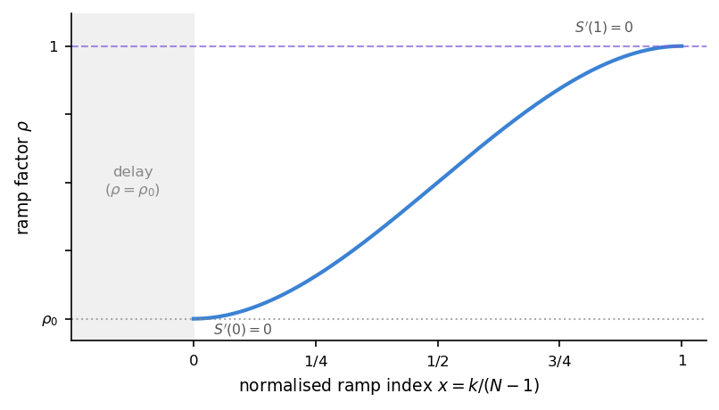
_images/continuation_ramp_smoothstep.png — Figure 10 Ramp factor \(\rho(k)\) as a function of the normalised index \(x=k/(N-1)\) for \(\rho_0=0\). The shaded region to the left represents the optional delay phase, during which \(\rho\) is held at \(\rho_0\). The zero-derivative conditions at \(x=0\) and \(x=1\) ensure a smooth entry into and exit from the active ramp.¶

Demagnetization ramp. When demag_ramp_N is set (demag driver), the demagnetization energy density \(W_{\mathrm{d}}\) ((124)) is multiplied by a prefactor \(\rho_{\mathrm{dem}}(s)\), which follows schedule (178) with \(\rho_0=\) demag_start_fraction, \(d=\) demag_ramp_delay, and \(N=\) demag_ramp_N:

(179)¶\[W_{\mathrm{d}} \;\leftarrow\; \rho_{\mathrm{dem}}(s)\,W_{\mathrm{d}}.\]

The prefactor is updated each step preamble by update_demag_ramp_factor and copied into the PETSc coefficient demag_ramp_constant before each weak-form assembly. While \(\rho_{\mathrm{dem}}<1\), the thermodynamic gate (phase E) is disabled: the energy baseline is shifting step by step, so a dissipation inequality on \(E_{\mathrm{gate}}\) is not meaningful until the full model is reached.

Zeeman ramp. When zeeman_ramp_N is set, the applied field is scaled as

(180)¶\[\mathbf{H}_{\mathrm{zee}}^\ast(s) = \rho_{\mathrm{zee}}(s)\,\mathbf{H}_{\mathrm{zee,orig}}^\ast,\]

following schedule (178) with \(\rho_0=\) zeeman_start_fraction, \(d=\) zeeman_ramp_delay, and \(N=\) zeeman_ramp_N. Unlike the demag ramp, the thermodynamic gate remains active during the Zeeman ramp: the applied-field change is accounted for by the external-work term \(W_{\mathrm{ext}}\) ((164)), which tracks the change in \(\mathbf{H}_{\mathrm{zee}}^\ast\) between the previous and current accepted steps.

Transition guard. When \(\rho\) reaches 1, _mark_continuation_transition records a transition event. On the next step preamble, before the \(\Delta t\)-retry loop, the solver applies a stabilization bundle to allow the system to equilibrate under the now fully-coupled model:

\(\Delta t^\ast\) is reduced by a factor _continuation_transition_dt_shrink_factor.
The history caps continuation_transition_dt_cap, thermo_dt_cap, and nonthermo_dt_cap are tightened to prevent immediate step-size recovery.
_bdf_active_order is reset to 1 for _continuation_transition_be_recovery_steps accepted steps, discarding the BDF2 history that was built under the partial model.
The thermodynamic baseline \(E^n_{\mathrm{gate}}\) and \(E^n_{\mathrm{phys}}\) are rebased to the current state, so the gate does not compare against pre-transition energies.
A reconcile window of _continuation_transition_reconcile_steps accepted steps begins, during which the thermodynamic gate and the atlas closure jump check remain suspended. The window decrements on each accept and the gates re-engage once it expires.

Physical steady-state stopping¶

When convergence_settings is provided, _check_physical_convergence tests for steady state after each accepted step. The two monitored quantities are:

Atlas-blended magnetization \(\mathbf{m}\) ((144)) — the Cartesian direction field reconstructed from both charts.
Physical energy \(E_{\mathrm{phys}}\) ((145)) — the total energy evaluated on the blended state.

These are used instead of the chart fields \((\mathbf{q}_A,\mathbf{q}_B)\) or \(E_{\mathrm{split}}\) because atlas closure (phase F) redistributes energy between the two chart representations without altering \(\mathbf{m}\), which would otherwise produce a spurious nonzero \(\Delta E_{\mathrm{split}}\) at a true steady state and reset the counter.

The first criterion measures the RMS rate of change of the magnetization direction. Let \(\Delta\mathbf{m}^n = \mathbf{m}^{n+1} - \mathbf{m}^n\) be the nodewise difference of the blended Cartesian fields at two consecutive accepted steps. The RMS rate is

(181)¶\[\dot{m}_{\mathrm{rms}} = \frac{1}{\Delta t^\ast} \sqrt{\frac{1}{N_{\mathrm{nodes}}} \sum_i |\Delta\mathbf{m}^n_i|^2}.\]

The second criterion measures the relative rate of change of \(E_{\mathrm{phys}}\):

(182)¶\[\dot{E}_{\mathrm{rel}} = \frac{\bigl|E_{\mathrm{phys}}^{n+1} - E_{\mathrm{phys}}^{n}\bigr|} {\Delta t^\ast\,\max\!\bigl(|E_{\mathrm{phys}}^{n+1}|,\,|E_{\mathrm{phys}}^{n}|,\,1\bigr)}.\]

Both criteria must be satisfied simultaneously at a given step. The steady-state counter increments when both hold and resets to zero when either fails. Termination is triggered once the counter reaches steady_steps consecutive accepted steps:

(183)¶\[\dot{m}_{\mathrm{rms}} < \tau_{\mathrm{m}} \quad \text{and} \quad \dot{E}_{\mathrm{rel}} < \tau_{E},\]

with \(\tau_{\mathrm{m}}=\) physical_tol_mdot_rms and \(\tau_{E}=\) physical_tol_edot.

A separate stagnation warning is emitted when the relative change in \(\|\mathbf{F}\|\) between consecutive accepted steps falls below stagnation_tol for stagnation_steps consecutive steps. This indicates that the algebraic residual has plateaued, which may or may not coincide with physical steady state; the warning is informational and does not trigger termination.

Configuration parameters¶

The table below groups configuration keys by subsystem. Keys marked internal are assigned in init_dynamic on the driver class and are not normally set in user input files. Default values refer to the demag/nodemag drivers unless noted; see Configuration reference for the full schema.

Subsystem	Keys	Role and typical defaults
Timestep bounds	`cfl_settings`: `CFL`, `dt_min`, `dt_max`, `smooth_factor`, `max_growth`, `min_shrink`, `error_headroom`, `error_rel_tol`, `error_abs_tol`	(176)–(174); defaults in `DEFAULT_CFL_SETTINGS` (e.g.\(\mathrm{CFL}=0.5\), \(\omega=0.6\)).
Retry limits	`max_retry`, `max_retry_thermo`, `outer_split_retry_before_dt_cut`	Δt-retry loop at fixed \(\Delta t^\ast\); thermo and operator-split counters are separate.
Residual gate	`nonlinear_residual_max_accept`, `nonlinear_residual_ema_factor`, `nonlinear_residual_gate_warmup_steps`, `nonlinear_residual_gate_floor`, `nonlinear_residual_dt_relax_max`	Build \(g_{\mathrm{res}}\) ((156)–(157)); EMA factor default \(8\), floor default \(10^{-6}\).
Residual backtrack (D1)	`_residual_backtracking_` (internal*)	Enabled by default; \(\sigma=1/2\), \(\lambda_{\min}=1/64\), at most six trials.
Merit / soft residual (D2/D3)	`_residual_merit_` (internal*)	Merit thresholds; D3 always caps `nonthermo_dt_cap` on soft accept.
Thermodynamic gate (E)	`thermo_use_split_energy`, `thermo_enable_physical_guard`, `thermo_defect_ema_factor`, `thermo_demag_energy_rel_floor`	(168); split energy selected by default (\(\chi_{\mathrm{split}}=\mathrm{true}\)).
Thermodynamic backtrack (E1)	`thermo_backtracking_enable`, `thermo_backtracking_shrink`, `thermo_backtracking_max_iter`, `thermo_backtracking_min_lambda`	Default \(\sigma=1/2\), eight trials, \(\lambda_{\min}=1/256\); failure rejects.
Demag operator split	`outer_split_max_iter`, `outer_split_tol_q`, `outer_split_tol_phi`, `enforce_outer_split_acceptance`	Phase (B), demag only; default \(\tau_q=5\times 10^{-3}\), \(\tau_\varphi=10^{-3}\).
Atlas radius	`atlas_qmax_guard`, `_atlas_qmax_guard_soft_factor` (internal)	Phase (C); hard limit \(g_{\mathrm{hard}} = f_{\mathrm{hard}}\, r_{\mathrm{guard}}\); re-evaluated after backtracking.
Closure jump	`_atlas_closure_jump_rel_tol`, `_atlas_closure_jump_abs_floor`, `_atlas_closure_jump_reject_factor` (internal)	Phase (F); (170)–(171).
Continuation ramps	`demag_ramp_N`, `zeeman_ramp_N`, `_continuation_transition_` (internal*)	Thermodynamic gate inactive while \(\lambda_{\mathrm{dem}}<1\); reconcile window after ramp completion.
Recovery after rejection	`be_recovery_steps_on_thermo`, `thermo_dt_cap`, `nonthermo_dt_cap` (runtime)	BDF1 windows; caps limit \(\Delta t^\ast\) regrowth after marginal failures.

Diagnostics¶

The dictionary state_monitor records:

Key	Quantity
`thermo_last_energy`	\(E^n_{\mathrm{gate}}\) at last acceptance
`thermo_last_energy_physical`	\(E^n_{\mathrm{phys}}\) at last acceptance
`last_residual_gate`	\(g_{\mathrm{res}}\) in (158)
`last_outer_split_q_defect`	\(\delta_q\) in (150)
`last_outer_split_phi_defect`	\(\delta_\varphi\) in (151) (demag)
`last_closure_jump_energy`	\(\Delta E_{\mathrm{closure}}\) in (169)
`last_thermo_backtracking_lambda`	\(\lambda\) when thermodynamic backtracking accepted the step
`last_temporal_error_norm`	\(e\) in (173)
`last_dt_cfl_cap`, `last_dt_thermo_cap`, `last_dt_error_target`	Components of (176)

Detailed thermodynamic logging is enabled by enable_thermo_diagnostics and thermo_diag_log_accepted in args_init_dyn.