Stereographic formulation
The LLG equation derived in Magnetization dynamics governs the time evolution of the reduced magnetization \(\mathbf{m}\in\mathcal{S}^2\). Cartesian parametrizations do not preserve the unit-length constraint \(|\mathbf{m}|=1\) intrinsically, while spherical coordinates enforce it by construction but introduce coordinate singularities at the two physically reachable poles \(\theta_0=0,\pi\). Stereographic projection resolves both issues simultaneously: the constraint is built into the parametrization, and the only singularity is moved to infinity, where it cannot be reached by any finite coordinate state [Horley et al., 2009, Rybakov et al., 2015].
This section develops the stereographic formulation of the LLG equation in three stages.
It first derives the single-chart map, including the forward and inverse transformations,
tangent map, conformal metric, and projected LLG system, and then identifies the remaining
conditioning issue near the projection pole. It next introduces the two-chart atlas that
removes this limitation. The section closes with the weak formulation assembled by Z-mag
at each time step, including the energy torque functional and the nondimensional chart
residual.
The normalized LLG equation (6) from Magnetization dynamics is recalled here for reference:
where \(\gamma_0\), \(\mu_0\), \(\alpha\), and \(\mathbf{H}_{\text{eff}}\) are defined in Magnetization dynamics and Micromagnetic energy.
Single-chart projection
Stereographic projection provides a two-coordinate representation of the reduced magnetization \(\mathbf{m}\in\mathcal{S}^2\) in which the unit-length constraint is built into the parametrization itself. This section develops the single-chart formulation, deriving the coordinate map, the associated tangent map and conformal metric, the projected form of the LLG equation, and the representation of the effective field in chart variables.
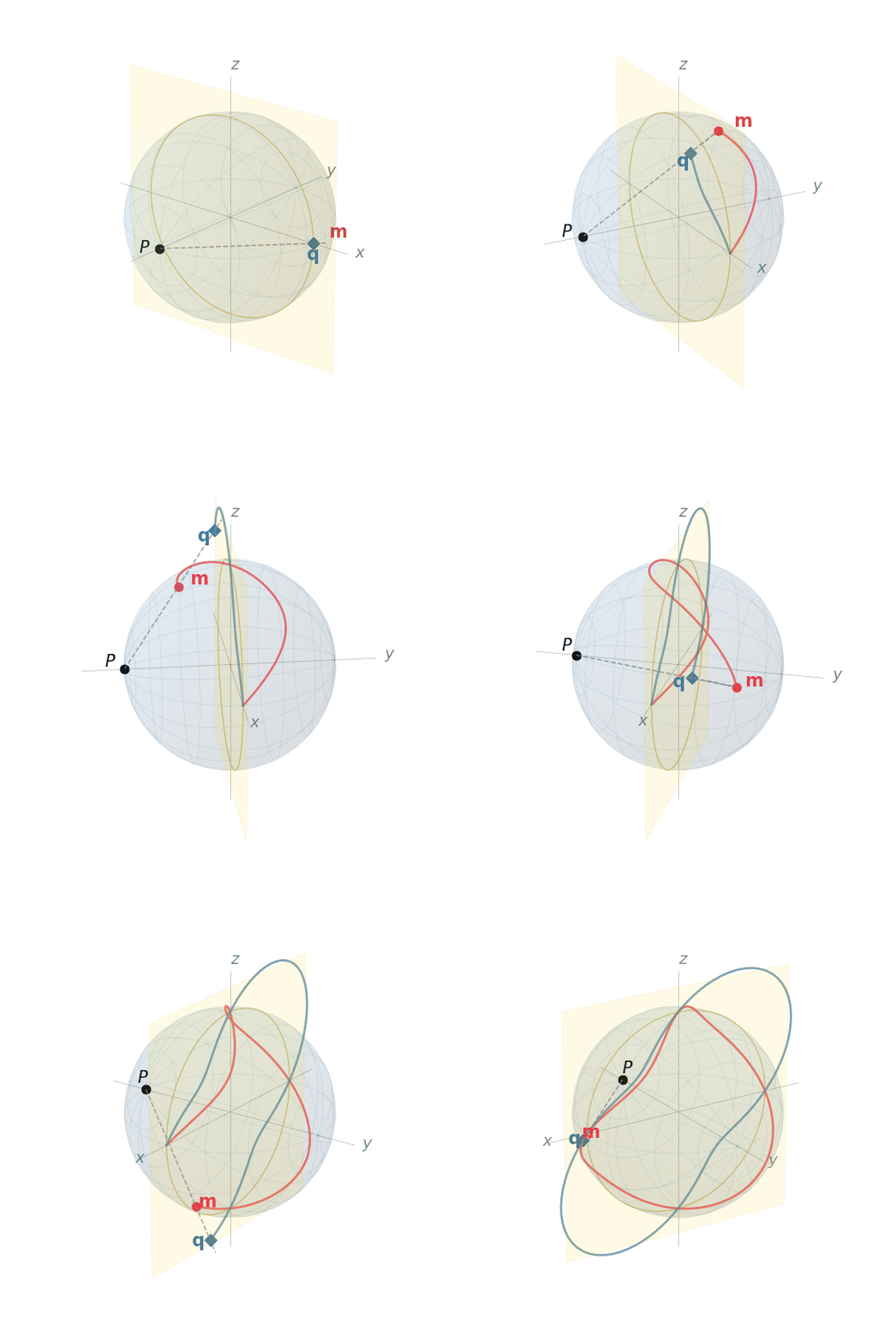
Figure 5 Stereographic projection from pole \(\mathbf{P}=(0,-1,0)\). As the magnetization \(\mathbf{m}\) (red) traces a trajectory on \(\mathcal{S}^2\), the projection line through \(\mathbf{P}\) maps \(\mathbf{m}\) to the equatorial coordinate \(\mathbf{q}\) (blue) on the plane \(y=0\). The coordinate \(|\mathbf{q}|\) remains moderate on the hemisphere opposite \(\mathbf{P}\) and grows without bound only as \(\mathbf{m}\to\mathbf{P}\).
Geometric construction
Let \(\mathbf{P}\in\mathcal{S}^2\) be a projection pole, and let \(\{\mathbf{e}_1,\mathbf{e}_2\}\) be an orthonormal basis of the plane through the origin perpendicular to \(\mathbf{P}\). As shown in Figure 5, for any \(\mathbf{m}\in\mathcal{S}^2\setminus\{\mathbf{P}\}\), the line passing through \(\mathbf{P}\) and \(\mathbf{m}\) intersects this equatorial plane at a unique point \(\mathbf{q}=(u,v)\in\mathbb{R}^2\). Solving for the intersection gives the forward map:
The denominator \(1-\mathbf{m}\cdot\mathbf{P}\) is strictly positive for all \(\mathbf{m}\neq\mathbf{P}\) and measures how close \(\mathbf{m}\) is to the pole.
The inverse map, recovering \(\mathbf{m}\) from \((u,v)\), is obtained by substituting the parametric form of the projection line back into the sphere equation \(|\mathbf{m}|=1\):
This formula reconstructs a unit vector for every finite \(\mathbf{q}\). To verify \(|\mathbf{m}|=1\) explicitly, note that \(\{\mathbf{P},\mathbf{e}_1,\mathbf{e}_2\}\) form an orthonormal basis, so
where the numerator identity \((1-r^2)^2 + 4r^2 = (1+r^2)^2\) follows from direct expansion. The mapping is therefore bijective between \(\mathbb{R}^2\) and \(\mathcal{S}^2\setminus\{\mathbf{P}\}\), with the pole \(\mathbf{P}\) corresponding to the limit \(|\mathbf{q}|\to\infty\). In contrast to spherical coordinates, where singularities occur at two finite parameter values (\(\theta_0=0,\pi\)), the stereographic singularity has been pushed to infinity and is therefore never reached by any finite coordinate state.
Tangent map
Since \(\mathbf{m}\) depends on time only through \(\mathbf{q}(t)\), the chain rule gives
The \(3\times 2\) matrix \(\mathcal{A}\) is called the tangent map. Differentiating (71) with respect to \(u\) by the quotient rule:
Grouping terms in \(\mathbf{P}\), \(\mathbf{e}_1\), and \(\mathbf{e}_2\):
The analogous calculation for \(v\) gives
Assembling both columns, the explicit tangent map is:
The columns of \(\mathcal{A}\) span the tangent space \(T_{\mathbf{m}}\mathcal{S}^2\): since \(|\mathbf{m}|^2=1\) implies \(\mathbf{m}\cdot\partial\mathbf{m}/\partial u=0\) and \(\mathbf{m}\cdot\partial\mathbf{m}/\partial v=0\), any variation \(\delta\mathbf{m}=\mathcal{A}\,\delta\mathbf{q}\) is automatically tangential to the sphere. The unit-length constraint is therefore built directly into the parametrization, so admissible first-order variations remain on \(\mathcal{S}^2\).
Conformal metric
The metric tensor induced by the parametrization is:
Because the metric \(\mathcal{P}\) is a scalar multiple of the identity, the stereographic map is conformal: angles between curves on the sphere are preserved by the projection, and both coordinate directions are scaled by the same local factor \(\sigma^2\). This follows directly from substituting (76) into \(\mathcal{A}^\text{T}\mathcal{A}\) and observing that the off-diagonal entries vanish identically.
The conformal factor \(\sigma^2=(2/(1+r^2))^2\) remains finite at \(r=0\),
corresponding to the antipodal point \(\mathbf{m}=-\mathbf{P}\), decreases monotonically as
\(r\) grows, and tends to zero as \(r\to\infty\) (i.e.as
\(\mathbf{m}\to\mathbf{P}\)). In the implementation, the same quantity is represented by
_sigma2().
The isotropic metric contrasts sharply with the spherical-coordinate metric
\(\mathcal{P}=\mathrm{diag}(1,\sin^2\theta_0)\), which degenerates along one direction as
\(\theta_0\to 0\) or \(\pi\).
LLG in stereographic coordinates
The derivation follows a standard projection strategy: substitute the chain rule (73) into the LLG equation (69), then project onto the coordinate plane by left-multiplying with \(\mathcal{A}^\text{T}\).
Step 1: substitute the chain rule. Replacing \(\partial_t\mathbf{m}\) by \(\mathcal{A}\,\partial_t\mathbf{q}\) in (69) gives
Step 2: left-multiply by \(\mathcal{A}^\text{T}\). Using \(\mathcal{A}^\text{T}\mathcal{A}=\sigma^2\mathbf{I}_2\) from (77):
Step 3: reduce the cross-product terms. Two identities simplify the right-hand side.
Identity 1. Let \(\mathbf{v}=(v_1,v_2)\in\mathbb{R}^2\). The vector \(\mathcal{A}\mathbf{v}=v_1\,\partial\mathbf{m}/\partial u + v_2\,\partial\mathbf{m}/\partial v\) is tangent to \(\mathcal{S}^2\) at the point \(\mathbf{m}\) because it is a linear combination of the basis vectors of \(T_{\mathbf{m}}\mathcal{S}^2\). The vector \(\mathbf{m}\times\mathcal{A}\mathbf{v}\) is therefore tangent as well: it is orthogonal to \(\mathbf{m}\) by construction, and hence lies in the tangent plane.
Consequently, \(\mathbf{m}\times\mathcal{A}\mathbf{v}\) can again be expanded in the same basis. The corresponding chart coordinates are obtained by applying \(\mathcal{A}^\text{T}\). A direct substitution of (76) gives
Writing this transformation in matrix form yields
Identity 2. Let \(\mathbf{w}\in\mathbb{R}^3\) be arbitrary. Decompose it into the sum of a component normal to the sphere \(\mathcal{S}^2\) and a component tangent to \(\mathcal{S}^2\) at the point \(\mathbf{m}\):
Here \(\mathbf{w}_{\perp}\) is the component normal to \(\mathcal{S}^2\), which is parallel to \(\mathbf{m}\), and \(\mathbf{w}_{//}\) is the component tangent to \(\mathcal{S}^2\). The normal contribution does not contribute to the cross product because \(\mathbf{w}_{\perp}\) is a scalar multiple of \(\mathbf{m}\):
since the cross product of any vector with itself is zero. Therefore
Because \(\mathbf{w}_{//}\) lies in the tangent plane, it can be expanded in the chart basis as \(\mathbf{w}_{//}=\mathcal{A}\mathbf{v}\) for some \(\mathbf{v}\in\mathbb{R}^2\). Applying Identity 1 gives
Moreover, because \(\mathbf{w}_{\perp}\) is parallel to \(\mathbf{m}\) while the columns of \(\mathcal{A}\) are tangent to the sphere, one has \(\mathcal{A}^\text{T}\mathbf{w}_{\perp}=0\). Hence
Thus \(\mathbf{v}=\sigma^{-2}\mathcal{A}^\text{T}\mathbf{w}\), and substitution into the previous relation yields
Step 4: assemble the projected equation. Applying Identity 1 to the damping term and Identity 2 to the precession term in (79):
Left-multiplying by \(-\mathbf{J}\) and using \(\mathbf{J}^{-1}=-\mathbf{J}\), \(\mathbf{J}^2=-\mathbf{I}_2\):
Defining the damping matrix \(\mathcal{L}(\mathbf{q})=\sigma^2(\alpha\mathbf{I}_2-\mathbf{J})\), the single-chart LLG in stereographic coordinates is
where
The determinant \(\det\mathcal{L}=\sigma^4(\alpha^2+1)>0\) is strictly positive for all finite \(\mathbf{q}\), so the system is well-posed and uniquely determines \(\partial_t\mathbf{q}\) at every point. In spherical coordinates, by contrast, \(\det\mathcal{L}=(1+\alpha^2)\sin^2\theta_0\) vanishes at the physically reachable poles.
Projected effective field
The right-hand side of (83) involves the projection \(\mathcal{A}(\mathbf{q})^\text{T}\mathbf{H}_{\text{eff}}\), where \(\mathbf{H}_{\text{eff}}\) is the sum of four contributions defined in Micromagnetic energy:
The anisotropy, Zeeman, and demagnetizing fields depend on \(\mathbf{m}\) but not on its spatial gradients. Their projected chart forces \(\mathcal{A}^\text{T}\mathbf{H}_{\text{ani}}\), \(\mathcal{A}^\text{T}\mathbf{H}_{\text{zee}}\), and \(\mathcal{A}^\text{T}\mathbf{H}_{\text{d}}\) are therefore obtained by pointwise multiplication of the Cartesian field by \(\mathcal{A}^\text{T}\), without involving spatial derivatives of the chart map.
The exchange contribution requires separate treatment. Its energy density \(A|\nabla\mathbf{m}|^2\) depends on spatial gradients of \(\mathbf{m}\), so expressing it in chart coordinates introduces both the conformal metric and an additional term arising from the spatial variation of the tangent basis. Applying the spatial chain rule \(\nabla\mathbf{m}=\mathcal{A}\nabla\mathbf{q}\) together with the metric (77) gives
so the exchange energy simplifies to
This conformally weighted Dirichlet functional is the natural analogue of the Cartesian exchange energy. Variational differentiation with respect to \(\mathbf{q}\) yields the projected exchange field:
The first term is a conformally weighted Laplacian arising from the first variation of (87). The correction \(\mathbf{Q}\) accounts for the curvature of the stereographic coordinate frame. Because the tangent basis \(\{\partial\mathbf{m}/\partial u,\partial\mathbf{m}/\partial v\}\) varies with \(\mathbf{q}\), differentiation of \(\mathcal{A}(\mathbf{q})\nabla\mathbf{q}\) produces additional terms that are absent in a flat parametrization. The correction vanishes whenever \(\nabla\mathbf{q}=0\), i.e. for spatially uniform magnetization.
This decomposition is mirrored in the implementation. The conformal metric is assembled by
P_mu_gamma(),
while the curvature term \(\mathbf{Q}\) is returned by
Q_mu().
Accordingly, the exchange contribution is written explicitly in the dynamic weak form, whereas the
anisotropy, Zeeman, and demagnetizing contributions enter through pointwise projections of their
Cartesian fields.
Summary and limitation
The single-chart stereographic formulation has several structural advantages over Cartesian and spherical-coordinate representations.
Constraint preservation by construction. The inverse map (71) sends every finite \(\mathbf{q}\) to a unit vector on \(\mathcal{S}^2\). The magnetization therefore satisfies \(|\mathbf{m}|=1\) identically, and the tangent-map relation (73) ensures that time variations remain tangent to the sphere.
Non-degenerate system matrix. The damping matrix (84) satisfies \(\det\mathcal{L}=\sigma^4(\alpha^2+1)>0\) for every finite \(\mathbf{q}\). The projected evolution equation is therefore well posed throughout the chart domain, in contrast to spherical-coordinate formulations whose system matrix degenerates at \(\theta_0=0,\pi\).
Isotropic conformal metric. The induced metric (77) has the form \(\mathcal{P}=\sigma^2\mathbf{I}_2\). Both coordinate directions are scaled by the same factor, so the chart introduces no directional bias in the differential operators. This isotropic structure simplifies the exchange contribution and avoids the directional degeneracy associated with spherical coordinates.
Fixed global basis. The tangent structure is encoded in the smooth map \(\mathcal{A}(\mathbf{q})\) rather than in nodewise orthonormal frames. A single pair \(\{\mathbf{e}_1,\mathbf{e}_2\}\) fixed in space is sufficient to define the chart over the whole domain.
The remaining limitation arises when the magnetization approaches the projection pole \(\mathbf{P}\). In that regime the coordinate radius satisfies \(|\mathbf{q}|\to\infty\), while the conformal factor in (77) tends to zero. The entries of the damping matrix (84) then become small in absolute value, whereas the exchange correction \(\mathbf{Q}\) in (88) becomes comparatively large. Trajectories that pass sufficiently close to the projection pole may therefore lead to ill-conditioned nonlinear systems, especially if the solution spends several successive time steps in that region. This limitation motivates the two-chart stereographic atlas introduced in the next section.
Two-chart formulation
As established in the preceding section, the single-chart construction maintains bounded coordinates and a well-conditioned system matrix throughout the hemisphere opposite the projection pole, but its conformal factor \(\sigma^2\) tends to zero as \(\mathbf{m}\to\mathbf{P}\). A trajectory that passes through or near the pole encounters coordinates of unbounded magnitude, reducing the entries of \(\mathcal{L}\) and amplifying the curvature correction \(\mathbf{Q}\) in (88). Introducing a second stereographic chart whose pole is placed at \(-\mathbf{P}\) ensures that every magnetization state is well-conditioned in at least one of the two charts. This section derives the unified parametrization, the conformal metric, the projected LLG and effective field in each chart, the weighted atlas combination, and the initialization procedure.
Geometric construction
Two stereographic charts, denoted A and B, are defined with projection poles \(\mathbf{P}\) and \(-\mathbf{P}\) respectively. Both share the equatorial plane through the origin perpendicular to \(\mathbf{P}\), spanned by the same orthonormal basis \(\{\mathbf{e}_1,\mathbf{e}_2\}\) as the single-chart construction; they differ only in the sign of the pole vector.
For any \(\mathbf{m}\in\mathcal{S}^2\), the chart-A coordinate radius satisfies \(|\mathbf{q}_A|\leq 1\) whenever \(\mathbf{m}\cdot\mathbf{P}\leq 0\) (the hemisphere opposite \(\mathbf{P}\)), while the chart-B radius satisfies \(|\mathbf{q}_B|\leq 1\) whenever \(\mathbf{m}\cdot\mathbf{P}\geq 0\) (the hemisphere opposite \(-\mathbf{P}\)). The two hemispheres thus provide complementary coverage: every direction that has large coordinates in one chart has bounded coordinates in the other. The charts overlap in the equatorial band \(|\mathbf{m}\cdot\mathbf{P}|\approx 0\), where both coordinate radii are of order unity (Figure 6).
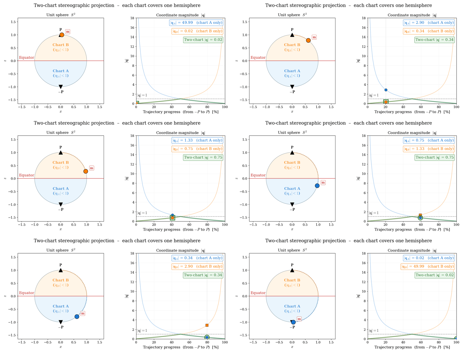
Figure 6 Complementary hemispheric coverage of the two-chart atlas. Left: a magnetization direction \(\mathbf{m}\) traverses a great circle; the shaded hemisphere indicates which chart keeps the stereographic radius bounded by \(|\mathbf{q}|\leq 1\). Right: the radii \(|\mathbf{q}_A|\) and \(|\mathbf{q}_B|\) each diverge near their respective poles, while the active chart remains bounded throughout the motion.
A unified parametrization is obtained by introducing a sign parameter \(s\in\{+1,-1\}\), with \(s=+1\) for Chart A and \(s=-1\) for Chart B. The inverse stereographic map then takes the single form
where \(\mathbf{q}=(u,v)\) and \(r^2=u^2+v^2\). The role of \(s\) is to switch the projection pole while leaving the planar coordinates unchanged. This is seen directly at the origin,
so \(\mathbf{q}=\mathbf{0}\) corresponds to opposite poles of \(\mathcal{S}^2\) in the two charts. As a result, the mapping \(\mathbf{q}\mapsto\mathbf{m}\) depends on the chart: the same planar coordinate \(\mathbf{q}\) represents different points on \(\mathcal{S}^2\) for different values of \(s\). Conversely, a given magnetization state \(\mathbf{m}\in\mathcal{S}^2\) is represented by two distinct coordinate vectors \(\mathbf{q}_A\) and \(\mathbf{q}_B\), one in each chart, as illustrated in Figure 7.
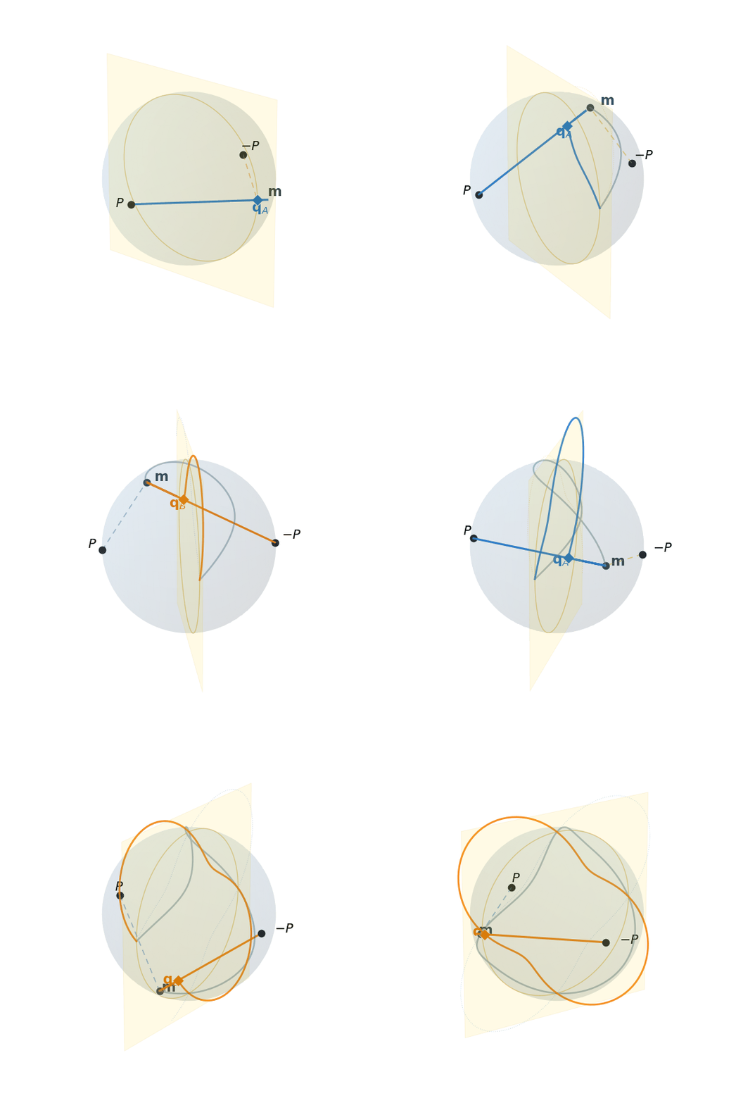
Figure 7 Dual-chart stereographic projection with antipodal poles \(\mathbf{P}=(0,-1,0)\) and \(-\mathbf{P}\). Both charts project \(\mathbf{m}\) onto the same equatorial plane \(y=0\); Chart~A (blue) and Chart~B (orange) use opposite projection poles. The active chart is shown with a solid ray from its pole through \(\mathbf{m}\) to the plane; the inactive chart is shown with a dashed segment from its pole to \(\mathbf{m}\).
Conformal metric
The metric tensor induced by the signed parametrization is \(\mathcal{P}(\mathbf{q},s)=\mathcal{A}(\mathbf{q},s)^\text{T}\mathcal{A}(\mathbf{q},s)\), where the tangent map \(\mathcal{A}(\mathbf{q},s)=\partial\mathbf{m}/\partial\mathbf{q}\) is obtained by differentiating (89):
Substituting into \(\mathcal{A}^\text{T}\mathcal{A}\), the cross-terms involving \(s\) cancel identically, and the metric reduces to
The metric is therefore independent of \(s\) and has the same functional form as in the single-chart case (77). It follows that the spatial chain rule \(\nabla\mathbf{m}=\mathcal{A}(\mathbf{q},s)\nabla\mathbf{q}\) and the gradient-norm identity \(|\nabla\mathbf{m}|^2=\sigma^2|\nabla\mathbf{q}|^2\) hold in either chart, so the exchange energy (87) retains the same conformally weighted Dirichlet structure in both.
LLG in each chart
The single-chart derivation of Section Single-chart projection carries over to each chart without modification. The projection steps (substituting the chain rule, left-multiplying by \(\mathcal{A}(\mathbf{q},s)^\text{T}\), and applying Identities 1 and 2) proceed identically, with the tangent map (91) replacing (76). The resulting projected LLG on chart \(s\) is
where the damping matrix is
The dependence on \(s\) appears exclusively in the off-diagonal entries. It reflects the reversal of orientation on the tangent plane when the projection pole changes sign: projection from \(\mathbf{P}\) and projection from \(-\mathbf{P}\) induce tangent bases of opposite handedness. The determinant \(\det\mathcal{L}=\sigma^4(\alpha^2+1)>0\) is strictly positive for all finite \(\mathbf{q}\) and both signs of \(s\); the sign parameter affects only the orientation of the off-diagonal precession term and leaves the well-posedness of the projected equation unchanged.
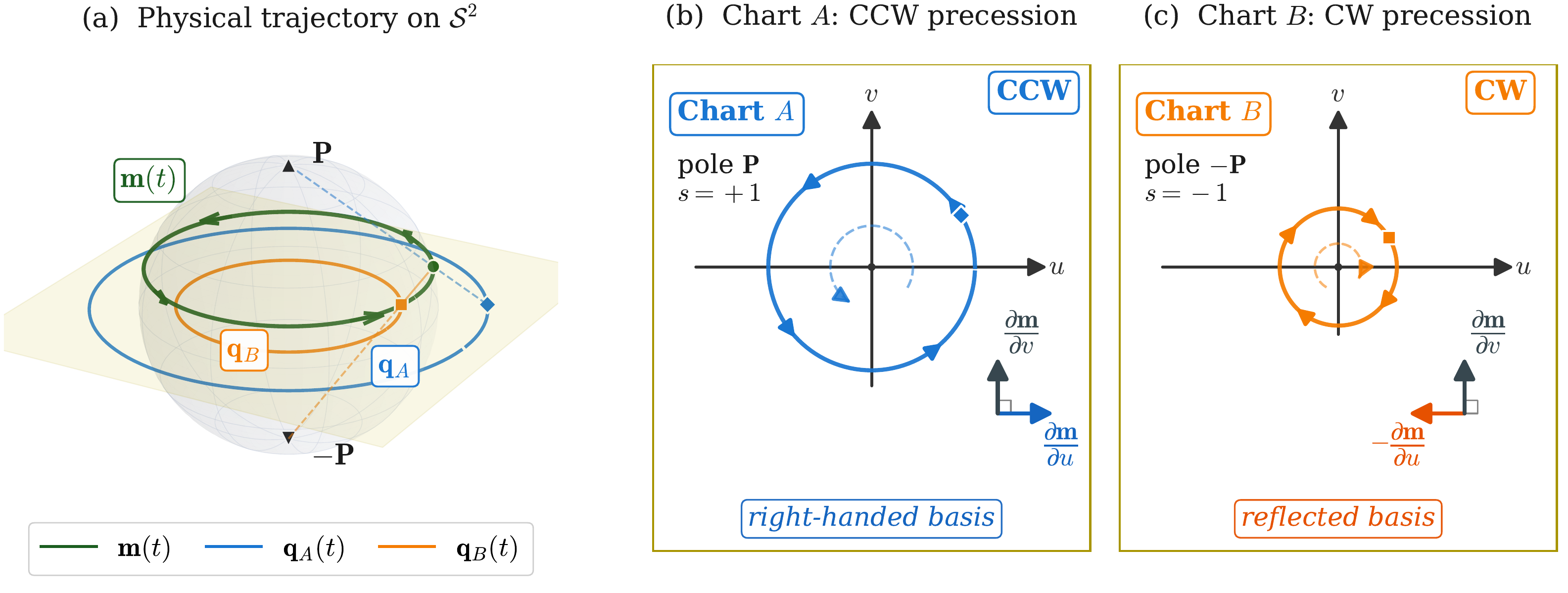
Figure 8 Handedness of the tangent basis in Charts A and B. Projection from \(\mathbf{P}\) (\(s=+1\)) and from \(-\mathbf{P}\) (\(s=-1\)) induce opposite orientations (counter-clockwise and clockwise, respectively), which is expressed as a sign reversal in the off-diagonal entries of \(\mathcal{L}(\mathbf{q},s)\) in (94).
Note
In the implementation, \(\sigma^2\) is regularized by a small floor value \(\sigma^2_{\mathrm{floor}}\) to prevent near-zero entries of \(\mathcal{L}\) in the case that coordinates approach the pole before a chart switch occurs:
This floor is active only in the inactive chart near its own pole; the active chart maintains \(\sigma^2\geq 1\) throughout its own hemisphere by construction.
Projected effective field
The right-hand side of (93) involves the projection \(\mathcal{A}(\mathbf{q},s)^\text{T}\mathbf{H}_{\text{eff}}\). Since the metric (92) is independent of \(s\), each contribution to the effective field takes the same form as in the single-chart case (85).
The anisotropy, Zeeman, and demagnetizing fields depend on \(\mathbf{m}\) but not on its spatial gradients, so their projections \(\mathcal{A}(\mathbf{q},s)^\text{T}\mathbf{H}_{\text{ani}}\), \(\mathcal{A}(\mathbf{q},s)^\text{T}\mathbf{H}_{\text{zee}}\), and \(\mathcal{A}(\mathbf{q},s)^\text{T}\mathbf{H}_{\text{d}}\) reduce to pointwise multiplication of each Cartesian field by \(\mathcal{A}(\mathbf{q},s)^\text{T}\).
The exchange contribution requires separate treatment because its energy density depends on spatial gradients of \(\mathbf{m}\). The variational derivative of (87) with respect to \(\mathbf{q}\) yields
where \(\mathbf{Q}\) is the curvature correction accounting for the spatial variation of the tangent basis. It involves only \(\mathbf{q}\), \(r^2\), and \(\nabla\mathbf{q}\) and carries no dependence on \(s\), so (95) is structurally identical to (88).
Atlas weights
Both chart fields \(\mathbf{q}_A\) and \(\mathbf{q}_B\) are carried as unknowns over the entire domain, each governed by (93) evaluated at \(s=+1\) and \(s=-1\) respectively. To maintain well-conditioned operators throughout the domain, cell-wise weights \(w_A(K)\) and \(w_B(K)\) are introduced that select the better-conditioned chart in each element and suppress the contribution of the ill-conditioned one.
The local conditioning of each chart is captured by the cell-averaged dot product
which measures the alignment of the magnetization with the projection axis in element \(K\). When \(\bar{s}_K\approx +1\), the magnetization is near the Chart-A pole \(\mathbf{P}\) and Chart A is ill-conditioned; when \(\bar{s}_K\approx -1\), Chart B is ill-conditioned instead. Given a threshold \(s_0\geq 0\) and a transition half-width \(\Delta s\geq 0\), the cell-wise weights are assigned as
Chart A is exclusively active (\(w_A=1\), \(w_B=0\)) when \(\bar{s}_K\leq-(s_0+\Delta s)\), i.e.where it is well-conditioned. Chart B is exclusively active in the symmetric case \(\bar{s}_K\geq s_0+\Delta s\). In the equatorial overlap band \(|\bar{s}_K|<s_0+\Delta s\), both charts are active and their weights vary linearly, reaching \(w_A=w_B=\tfrac{1}{2}\) at \(\bar{s}_K=0\). The parameter \(s_0\) sets the width of the flat equatorial region in which both charts remain comparably weighted, while \(\Delta s\) controls the steepness of the transition. The resulting weight functions are illustrated in Figure 9.
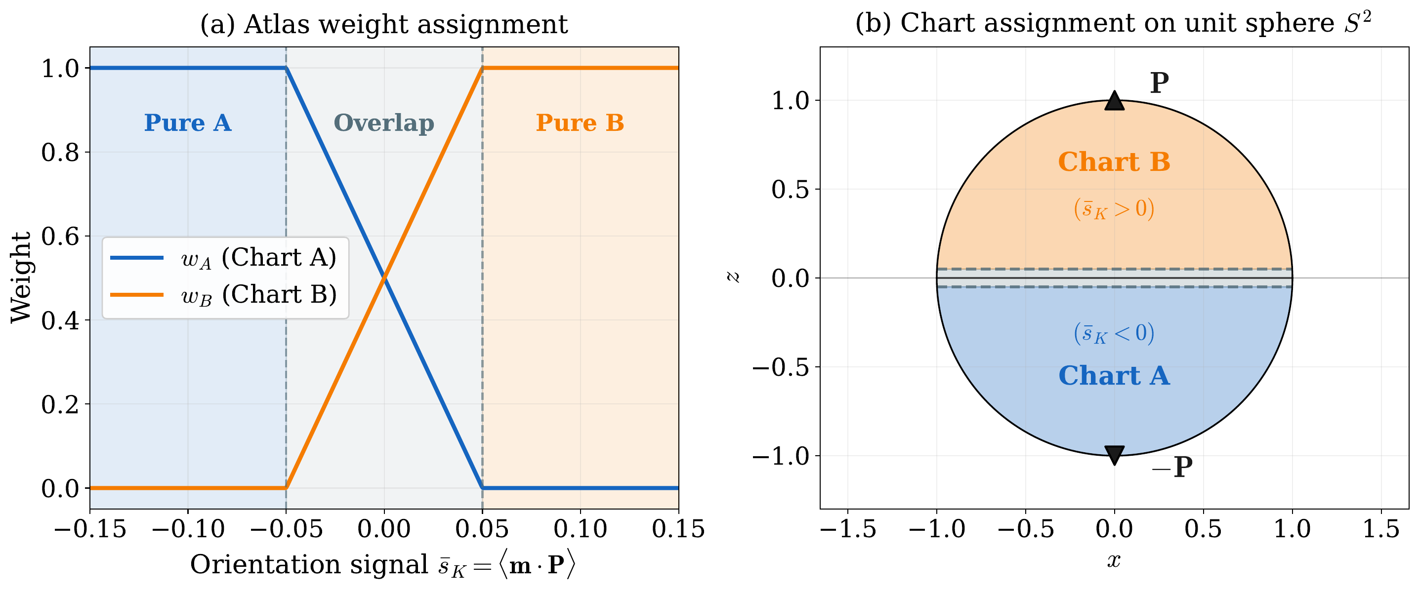
Figure 9 Atlas weight functions \(w_A\) and \(w_B\) from (97) as functions of \(\bar{s}_K\). Chart~A is exclusively active near \(\mathbf{m}\approx-\mathbf{P}\), Chart~B near \(\mathbf{m}\approx+\mathbf{P}\), with a linear transition through the equatorial overlap band of half-width \(s_0+\Delta s\).
Since the two hemispheres are complementary, at least one chart satisfies \(|\mathbf{q}|\leq 1\) and \(\sigma^2\geq 1\) for any \(\mathbf{m}\in\mathcal{S}^2\), ensuring that the active chart’s damping matrix (94) remains non-degenerate throughout the simulation. How these weights enter the assembled weak form is detailed in the Weak formulation section.
Weak formulation
This section derives the Galerkin weak form of the stereographic LLG equations that
Z-mag assembles at each time step
([Yi and Xu, 2014], [Abert, 2019]). The effective field
\(\mathbf{H}_\text{eff}\) is defined by (18) in Micromagnetic energy.
The demagnetizing variant additionally solves the Fredkin–Koehler magnetostatic subproblem
for \(\varphi\), described in Magnetostatics, and couples
\(\mathbf{H}_\text{d}=-\nabla\varphi\) back into the residual. Time discretization
(BDF formulas, timestep control, acceptance gates, and the SNES solve) is presented later
on this page in the Time discretization section; throughout this section
the time derivative \(\partial_t\mathbf{q}\) is kept in continuous form.
Galerkin projection
The strong-form LLG in chart coordinates for sign \(s\in\{+1,-1\}\) is (93), with the sign-dependent damping matrix (94). Let \(\mathbf{v}\in [H^1(\Omega_{\mathrm m})]^2\) be a vector-valued test function, where \(H^1(\Omega_{\mathrm m})\) denotes the Sobolev space of functions whose first derivatives are square-integrable on \(\Omega_{\mathrm m}\). Multiplying (93) by \(\mathbf{v}\) and integrating over \(\Omega_{\mathrm{m}}\) yields
The right-hand side is rewritten in terms of the total energy by substituting the definition of the effective field from Micromagnetic energy: the normalized negative variational derivative of the total micromagnetic energy with respect to \(\mathbf{m}\):
so that \(\mathcal{A}^{\mathrm{T}}\mathbf{H}_{\text{eff}}\) on the right-hand side of (98) represents the torque projected onto chart coordinates. Since \(\mathbf{m}=\mathbf{m}(\mathbf{q},s)\), a perturbation \(\delta\mathbf{q}=\mathbf{v}\) induces a tangent displacement \(\delta\mathbf{m}=\mathcal{A}(\mathbf{q},s)\,\mathbf{v}\). By the chain rule, the variational derivative of the energy with respect to the chart coordinate \(\mathbf{q}\) is therefore
where the second step uses (99). Solving for \(\gamma_0\mu_0\,\mathcal{A}^{\mathrm{T}}\mathbf{H}_{\text{eff}}\) and substituting into (98) yields
The right-hand side is a Gateaux derivative: for any energy functional \(\mathcal{E}[\mathbf{q}]\), the expression \(\delta\mathcal{E}[\mathbf{v}]\equiv\int(\delta\mathcal{E}/\delta\mathbf{q})\cdot\mathbf{v}\,dV\) is the directional derivative of \(\mathcal{E}\) at \(\mathbf{q}\) in the direction \(\mathbf{v}\). The four contributions to \(\mathcal{E}_{\mathrm{SI}}\) are derived in turn below.
The anisotropy, Zeeman, and demagnetizing energies depend on \(\mathbf{q}\) only through the pointwise evaluation \(\mathbf{m}(\mathbf{q},s)\) and carry no dependence on \(\nabla\mathbf{q}\), so their Gateaux derivatives are local in space. A perturbation \(\delta\mathbf{q}=\mathbf{v}\) induces a tangent displacement \(\delta\mathbf{m}=\mathcal{A}(\mathbf{q},s)\,\mathbf{v}\); the chain rule gives
for any integrand \(e\) differentiable in \(\mathbf{m}\) and independent of \(\nabla\mathbf{q}\). The exchange term requires separate treatment because the stereographic exchange energy (87) depends on \(\nabla\mathbf{q}\) and its Gateaux derivative involves integration by parts.
Anisotropy
From (12), the SI anisotropy integrand is
Its partial derivative with respect to \(\mathbf{m}\) is
Substituting into (102) gives
The factor \(\mathcal{A}(\mathbf{q},s)^{\mathrm{T}}\mathbf{e}_{\mathrm{ua}}\) is the projection of the easy-axis direction onto the chart tangent plane.
Zeeman
From (15), the SI Zeeman integrand is
with the applied field \(\mathbf{H}_{\mathrm{zee}}\) prescribed and independent of \(\mathbf{m}\). Its partial derivative is
Substituting into (102):
Demagnetization
From (17), the SI demagnetizing integrand is
where \(\mathbf{H}_{\mathrm{d}}=-\nabla\varphi\) and \(\varphi\) is determined by a separate magnetostatic subproblem (see Magnetostatics). Treating \(\varphi\) as fixed when varying \(\mathbf{q}\), the partial derivative with respect to \(\mathbf{m}\) is
Substituting into (102):
Exchange
The exchange energy (87) depends on \(\nabla\mathbf{q}\), so (102) does not apply and integration by parts is required. The stereographic exchange energy recasts (10) as
where the conformal factor \(\sigma^2(\mathbf{q})=(2/(1+r^2))^2\) from (77) weights the Dirichlet energy by the stereographic metric. The first variation in the direction \(\mathbf{v}\) decomposes into two terms:
The first integral arises from varying \(\nabla\mathbf{q}\) at fixed \(\mathbf{q}\); the second from the implicit dependence of \(\sigma^2\) on \(\mathbf{q}\). Defining the configurational stress tensor
the first integral in (106) reads \(\int_{\Omega_{\mathrm m}}\boldsymbol{\Pi}_\mu:\nabla\mathbf{v}\,dV\). Applying Green’s first identity gives
The boundary trace evaluates to
which is proportional to the normal derivative of the chart field. Under the natural
Neumann boundary condition (flag NeumannBC = True),
which is the chart-coordinate form of Brown’s exchange boundary condition \(A\,\partial_{\mathbf{n}}\mathbf{m}=\mathbf{0}\) ((21)), the surface integral in (108) vanishes. Collecting the volume divergence term from (108) and the \(\sigma^2\)-variation term from (106) into the curvature correction \(\mathbf{Q}_\mu\) from (88) yields the symmetric exchange weak form
where
is the curvature correction (from (88)) accounting for the spatial variation of the stereographic frame. The first term in (109) is the bilinear gradient coupling between \(\mathbf{q}\) and \(\mathbf{v}\) weighted by the conformal metric; the second is a nonlinear correction that vanishes for spatially uniform magnetization (\(\nabla\mathbf{q}=\mathbf{0}\)).
Total weak form
Substituting the four Gateaux derivatives (103), (104), (105), and (109) into the right-hand side of (101), and noting that \(-\gamma_0 M_{\mathrm{s}}^{-1}\,\delta\mathcal{E}_{\mathrm{SI}}/\delta\mathbf{q}\) collects all four energy torques, yields the complete SI weak form for chart \(s\), satisfied for every \(\mathbf{v}\in[H^1(\Omega_{\mathrm{m}})]^2\):
The left-hand side is the inertia-like damping term from the projected LLG. The right-hand side collects the four energy torques derived above. No boundary terms appear because the natural Neumann condition eliminates the exchange surface integral.
Atlas residual
The weak form (111) is expressed in SI units. To obtain the residual
that Z-mag assembles internally, the spatial scaling relations
(23) from Micromagnetic energy are supplemented by a temporal
scale. The nondimensional time is defined by
whose unit \((\mu_0\gamma_0 M_{\mathrm{s}1})^{-1}\) is the precession period of the reference material. Substituting (112) and (23) into (111) and dividing through by \(\mu_0\gamma_0 M_{\mathrm{s}1}^2\,\ell_{\mathrm{ex}1}^3\) eliminates all dimensional prefactors.
The assembled nonlinear system couples two types of residual blocks. The chart blocks \(\mathcal{F}_A(\mathbf{v})\) and \(\mathcal{F}_B(\mathbf{v})\) enforce the stereographic LLG for each chart; they are always present. When the self-consistent stray-field contribution is included, a magnetostatic block \(F_\varphi(v_\varphi)\) is added, which enforces consistency between the scalar magnetostatic potential \(\varphi\) and the current atlas state. The full nonlinear system is
where \(F_\varphi = 0\) when the stray-field contribution is absent. The two block types are derived below.
Chart blocks
The two charts carry independent unknown fields \(\mathbf{q}_A\) and \(\mathbf{q}_B\) over the entire domain \(\Omega_{\mathrm{m}}\). After the scaling of the preceding paragraph, each chart is weighted by \(w_s\) ((97)) and the material ratio \(M_{\mathrm{s}}^\ast\), and the time derivative is written as \(\dot{\mathbf{q}}_s\equiv\partial\mathbf{q}_s/\partial t^\ast\). This yields the chart residual for sign \(s\in\{+1,-1\}\):
The first line is the inertia-damping term; lines 2–5 are the nondimensional,
atlas-weighted Gateaux derivatives of the four energy contributions already
assembled in (111). The scalar \(\lambda_{\mathrm{dem}}\in[0,1]\) is
the continuation ramp factor
(demag_ramp_constant), set to unity once the ramp is complete. On heterogeneous
domains, \(M_{\mathrm{s}}^\ast\), \(A^\ast\), and \(K^\ast\) are
piecewise-constant material ratio fields ((24)).
Collecting lines 2–5 defines the energy torque functional
where \(\delta\mathcal{E}_{\mathrm{SI}}[\mathbf{v}]\) is the SI Gateaux derivative introduced in the Galerkin projection above, evaluated at sign \(s\) through \(\mathcal{A}(\mathbf{q}_s,s)\). The prefactor carries the nondimensionalisation of (111) together with the atlas weight \(w_s\). The chart residual then takes the compact form
Magnetostatic block
When the stray-field energy term is active, the scalar magnetostatic potential
\(\varphi\) ((16)) becomes a third unknown. The potential satisfies the
Poisson equation \(\Delta\varphi = \nabla\cdot\mathbf{M}\) derived in
Magnetostatics ((51)). In the operator-splitting
scheme implemented in Z-mag, \(\varphi\) is not solved simultaneously with the
LLG Newton iteration. Instead, at the start of each accepted time step, the
Fredkin–Koehler subproblem (Magnetostatics) is solved for a frozen
atlas state to produce a reference potential \(\varphi_{\mathrm{ref}}\). Within
the subsequent SNES Newton iteration, the block \(F_\varphi\) then constrains
the Newton iterate \(\varphi\) to remain consistent with \(\varphi_{\mathrm{ref}}\):
This is a Laplace equation for the difference \(\varphi - \varphi_{\mathrm{ref}}\), which has the unique solution \(\varphi = \varphi_{\mathrm{ref}}\) (up to a constant) under natural boundary conditions. The block therefore acts as a consistency constraint: it drives the Newton iterate \(\varphi\) toward the reference potential produced by the outer magnetostatics solve without re-solving the full Fredkin–Koehler system at each Newton step. The full nonlinear system \(\mathcal{F}_A + \mathcal{F}_B + F_\varphi = 0\) is assembled as a single coupled problem and passed to PETSc SNES; the demag operator-split loop, acceptance logic, and inner Jacobian structure are described in Solver algorithms.
The magnetization sourcing \(\varphi_{\mathrm{ref}}\) is the atlas-blended field
using the cell weights \(w_A\), \(w_B\) from (97).
Stored energy
Assembling (116) requires the energy torque
\(\mathcal{G}_s\) ((115)). Rather than differentiating
\(\mathcal{E}_{\mathrm{SI}}\) directly, Z-mag builds \(\mathcal{G}_s\) from
the Gateaux derivative of the stored energy
with nondimensional densities \(W_i\) chosen so that
at fixed \(\varphi\) and chart sign \(s\). Each \(W_i=\tfrac{1}{2}e_i\) is half the corresponding integrand of \(\mathcal{E}^\ast\) ((31)); the variational checks are given in Micromagnetic energy. In chart coordinates,
In the two-chart implementation, each density is multiplied by the atlas weight \(w_s\) before integration. The Gateaux derivative \(\delta(w_s W_i)[\mathbf{v}]\) is obtained term by term as follows:
Exchange (\(W_{\mathrm{ex}}\)). Assembled directly from (109), because the gradient dependence of \(W_{\mathrm{ex}}\) through the conformal metric \(\mathcal{P}_\mu\) is not captured by differentiating the density alone.
Anisotropy (\(W_{\mathrm{ani}}\)) and Zeeman (\(W_{\mathrm{zee}}\)). Obtained from the Gateaux derivative of the weighted densities \(w_s W_{\mathrm{ani}}\) and \(w_s W_{\mathrm{zee}}\). Both depend on \(\mathbf{q}_s\) only through the pointwise map \(\mathbf{m}(\mathbf{q}_s,s)\) and carry no \(\nabla^\ast\mathbf{q}_s\), so the chain rule through the stereographic map is exact.
Stray field (\(W_{\mathrm{d}}\)). Assembled from the projected demagnetizing field with \(\varphi\) held fixed while \(\mathbf{q}_s\) is varied, as in (105).
The same weighted \(W_i\) are integrated at run time for energy monitoring; see Solver algorithms for the thermodynamic gate.
Time discretization
The chart fields \(\mathbf{q}_s(\mathbf{x},t)\) are already discretized in space by the finite-element mesh: expanding in the Lagrange nodal basis reduces the unknowns to time-dependent coefficient vectors \(\{q_{s,i}(t)\}\), and substituting into (116) yields a system of ordinary differential equations (ODEs) for those coefficients. The only remaining continuous variable is time. This section approximates the time derivative by a backward-differentiation formula, justifies the implicit formulation on stiffness grounds, and derives the continuous energy decay identity together with its discrete analogue. Timestep control and the operator-splitting loop for the demag driver are documented in Solver algorithms.
Backward-differentiation formulas
The inertia-damping term in (116) involves the time derivative \(\dot{\mathbf{q}}_s\), which is approximated by expressing it at the new time level \(t^{n+1}\) as a linear combination of the solution at \(t^{n+1}\) (unknown) and at the two most recently accepted times \(t^n\) and \(t^{n-1}\) (known). A backward-differentiation formula (BDF) determines the coefficients by requiring exact reproduction of the derivative for polynomials up to a given degree:
Substituting (125) into (116) converts the ODE for the nodal coefficients into a nonlinear algebraic equation for \(\mathbf{q}_s^{n+1}\), with the history values treated as constants. Two orders are used.
First-order (BDF1). Setting \((c_0,c_1,c_2)=(1,-1,0)\) gives the backward-Euler formula \(\dot{\mathbf{q}}_s\approx(\mathbf{q}_s^{n+1}-\mathbf{q}_s^n)/\Delta t^\ast\). BDF1 is first-order accurate and requires only one history level; it is therefore always available. The integrator begins in BDF1 mode and falls back to it after any rejection event or continuation-ramp transition that may have invalidated the two-step history.
Variable-step BDF2. When two consecutive accepted steps are available, the accuracy is raised to second order. Because the timestep controller adjusts \(\Delta t^\ast\) at every step, consecutive intervals are generally of different lengths. The coefficients must account for the ratio \(r=\Delta t^\ast/\Delta t^{n-1}\) of the current to the previous accepted step; requiring exact reproduction of the derivative for quadratic functions of time on this non-uniform spacing gives
For equal step sizes (\(r=1\)) these reduce to the standard coefficients \((3/2,\,-2,\,1/2)\). BDF2 is second-order accurate and is activated automatically once two consecutive accepted steps are available without an intervening restart.
Embedded temporal defect. A practical step-size controller requires an estimate of the local truncation error without solving an additional system. The BDF2 and backward-Euler formulas applied to the same snapshot history give rates that differ by a term of order \(\Delta t^2\) for smooth trajectories; their difference therefore measures how much the second-order formula corrects the first-order one. The estimate is formed on the atlas-blended magnetization \(\mathbf{m}\) ((118)) rather than on the raw chart coordinates, so that the error signal is chart-independent:
The root-mean-square (RMS) norm of \(\mathbf{e}_{\mathrm{temp}}\), normalised by the number of degrees of freedom, feeds the error-based timestep controller (Solver algorithms, (173)); in BDF1 mode no embedded estimate is available.
A-stability and stiffness
The ODE system for the nodal coefficients of (116) is stiff: it contains modes that evolve on widely separated timescales. The source of stiffness is the exchange Laplacian. The eigenvalues of the discrete operator \(-A^\ast\nabla^2\) form a spectrum ranging from values of order unity, associated with long-wavelength spatial variations (e.g.slow domain-wall displacement or uniform precession), up to a maximum that scales as
where \(h\) is the element size in the nondimensional units of (112). This largest eigenvalue governs fine-scale spatial oscillations near the mesh scale, which damp out on a timescale of order \(h^2/A^\ast\). Accurate resolution of any non-uniform magnetization structure — domain walls, vortex cores, or skyrmion profiles — requires \(h\) to be a fraction of the exchange length (i.e.a fraction of unity in the nondimensional system), so \(|\lambda_{\max}|\) is several orders of magnitude larger than the eigenvalues that govern the physically observable dynamics (e.g.magnetization switching or domain-wall nucleation).
For an explicit time-stepping scheme, numerical stability requires the timestep to satisfy \(\Delta t^\ast \lesssim h^2/A^\ast\) [Hairer and Wanner, 1996]. This constraint tightens quadratically as the mesh is refined, forcing the integrator to resolve mesh-scale dissipation events that are irrelevant to the physical quantities of interest.
An implicit scheme avoids this restriction by evaluating the energy-torque right-hand side of (116) at the unknown time level \(t^{n+1}\) rather than at the accepted level \(t^n\). The stiff exchange modes then enter the nonlinear algebraic system solved at each step, so their stabilization is delegated to the Newton–Krylov iteration (described in Solver algorithms) rather than imposed as an upper bound on \(\Delta t^\ast\).
More precisely, a time-stepping method is A-stable if, for every linear test equation \(\dot{y}=\lambda y\) with \(\operatorname{Re}(\lambda)<0\), the numerical solution remains bounded at any step size [Hairer and Wanner, 1996]. The LLG satisfies this condition: the damping parameter \(\alpha>0\) ensures that every mode of the linearized system decays in time, so all eigenvalues have strictly negative real part. A-stability therefore guarantees bounded numerical solutions for every spatial mode, including the stiffest exchange mode (128), at any step size. Both BDF1 (backward Euler) and BDF2 satisfy this condition. By Dahlquist’s second barrier [Hairer and Wanner, 1996], no A-stable linear multistep method can exceed second order, so BDF2 is the highest-order scheme of this class and the natural upper bound for the adaptive integrator.
Energy decay and discrete energy balance
A-stability ensures bounded amplitudes for all spatial modes at any step size, but places no constraint on the sign of the energy increment \(\Delta\mathcal{E}_{\mathrm{sol}}\) at a finite step. The energy-decay identity (130) below provides that constraint for the continuous and semi-discrete systems; the remainder of this section establishes its discrete counterpart.
Continuous and semi-discrete decay. The continuous LLG is dissipative: Gilbert damping is the sole dissipation mechanism, and every non-stationary trajectory satisfies \(d\mathcal{E}/dt\leq 0\) [Abert, 2019]. After Galerkin finite-element assembly, the same inequality holds for the semi-discrete system, where the spatial degrees of freedom are finite-element nodal values but time remains a continuous variable [Baňas, 2019, Kružík and Prohl, 2006]. The key property that makes this possible is that the time derivative \(\dot{\mathbf{q}}_s\) of any nodal coefficient vector belongs to the same finite-element space \(V_h\), and is therefore an admissible test function in the chart residual (116).
Setting \(\mathbf{v}=\dot{\mathbf{q}}_s\) in (116) and using \(\mathcal{F}_s(\dot{\mathbf{q}}_s)=0\) (the residual vanishes on a solution) yields
The second term equals \(d\mathcal{E}_{\mathrm{sol}}/dt^\ast\) because \(\mathcal{G}_s\) is by construction the Gateaux derivative of \(\mathcal{E}_{\mathrm{sol}}\) with respect to \(\mathbf{q}_s\) ((119), (120)): evaluating it in the direction \(\dot{\mathbf{q}}_s\) gives exactly the rate of change of \(\mathcal{E}_{\mathrm{sol}}\) along the trajectory, by the chain rule.
The first term reduces to a purely dissipative contribution. The damping matrix (94) decomposes as \(\mathcal{L}=\alpha\sigma^2\mathbf{I}_2+s\sigma^2\mathbf{J}\), where \(\mathbf{J}=\bigl(\begin{smallmatrix}0&1\\-1&0\end{smallmatrix}\bigr)\) is skew-symmetric, i.e.\(\mathbf{J}^\mathrm{T}=-\mathbf{J}\). For any vector \(\mathbf{x}\), the quadratic form \(\mathbf{x}^\mathrm{T}\mathbf{J}\mathbf{x}=0\) identically, because \(\mathbf{x}^\mathrm{T}\mathbf{J}\mathbf{x}=-\mathbf{x}^\mathrm{T}\mathbf{J}^\mathrm{T}\mathbf{x} =-\mathbf{x}^\mathrm{T}\mathbf{J}\mathbf{x}\), which forces the expression to zero. Consequently the skew-symmetric, precession part of \(\mathcal{L}\) contributes nothing to the quadratic form \(\dot{\mathbf{q}}_s^\mathrm{T}\mathcal{L}\dot{\mathbf{q}}_s\), and only the symmetric damping part \(\alpha\sigma^2\mathbf{I}_2\) survives. In physical terms, the precession torque \(\mathbf{m}\times\mathbf{H}_\text{eff}\) is orthogonal to \(\partial_t\mathbf{m}\) and therefore does no work on the magnetization; only the dissipative component of \(\mathcal{L}\) contributes to the power balance. Equation (129) thus becomes
Summing over both charts \(s\in\{+1,-1\}\) and noting that all integrands are non-negative, the left-hand side is non-negative and its equality to \(-d\mathcal{E}_{\mathrm{sol}}/dt^\ast\) yields the energy-decay identity:
with equality only at stationary states (\(\dot{\mathbf{q}}_s\equiv 0\) for both charts). This identity is exact for both the continuous and the Galerkin semi-discrete systems: because \(\dot{\mathbf{q}}_s\) lies in \(V_h\), every step in the derivation holds algebraically in the finite-element space, and spatial discretization introduces no error.
Discrete energy balance. The derivation of (130) requires \(\dot{\mathbf{q}}_s\) to be an admissible test function and to satisfy the chain-rule identity \(\mathcal{G}_s[\dot{\mathbf{q}}_s]=d\mathcal{E}_{\mathrm{sol}}/dt^\ast\). Both conditions hold at the semi-discrete level, where \(\dot{\mathbf{q}}_s\) is the genuine time derivative of a continuous trajectory. Once time is also discretized, \(\dot{\mathbf{q}}_s\) is replaced by the BDF approximation (125), i.e.the linear combination \((c_0\,\mathbf{q}_s^{n+1}+c_1\,\mathbf{q}_s^n+c_2\,\mathbf{q}_s^{n-1})/\Delta t^\ast\). This linear combination is a vector of fixed real numbers formed from accepted nodal values at three time levels; it is not the time derivative of any continuous curve. As a consequence, evaluating \(\mathcal{G}_s\) on this vector no longer yields \(d\mathcal{E}_{\mathrm{sol}}/dt^\ast\) via the chain rule; the two terms in (129) — the damping integral and the energy rate — no longer sum to zero at a given discrete step. The relevant quantity at the discrete level is therefore the finite energy increment \(\Delta\mathcal{E}_{\mathrm{sol}}^{n+1}=\mathcal{E}_{\mathrm{sol}}^{n+1}-\mathcal{E}_{\mathrm{sol}}^{n}\) over \([t^n,t^{n+1}]\), and its sign is no longer guaranteed to be non-positive. Two independent sources contribute to the departure from exact decay:
Temporal truncation error. The BDF stencil reproduces the time derivative exactly only for polynomials up to degree \(p\), where \(p\) is the BDF order (\(p=1\) for BDF1, \(p=2\) for BDF2). Applied to the actual nonlinear trajectory, it introduces a local truncation error of order \(O(\Delta t^{p})\), which propagates into \(\Delta\mathcal{E}_{\mathrm{sol}}^{n+1}\). The BDF formulas are selected for their A-stability on the stiff exchange spectrum (128), not for any property of energy preservation.
Nonlinear solver residual. The discrete chart residual (134) is a nonlinear algebraic equation for \(\mathbf{q}_s^{n+1}\), solved at each step by PETSc SNES. The solver terminates when the residual norm \(\|\mathbf{F}\|\) falls below a prescribed tolerance, so the accepted iterate satisfies the equation only approximately. The resulting defect \(\|\mathbf{F}\|>0\) introduces an additional imbalance in \(\Delta\mathcal{E}_{\mathrm{sol}}^{n+1}\) that is independent of, and additive to, the temporal truncation error.
Dissipation and external work. The physical reference for the energy balance over \([t^n,t^{n+1}]\) consists of two quantities: the energy removed by Gilbert damping and the energy injected by any change in the applied field. The first is obtained by integrating the right-hand side of (130) over the step, with the continuous \(\dot{\mathbf{q}}_s\) replaced by the BDF approximation (125):
where \(\dot{\mathbf{q}}_s\) is the BDF approximation (125) evaluated at the accepted iterate. Because \(\alpha>0\) and all other factors are non-negative, \(D_q\geq 0\): Gilbert damping can only remove energy from the system.
A second contribution arises when the applied Zeeman field changes between \(t^n\) and \(t^{n+1}\). The Zeeman energy density \(W_{\mathrm{zee}}=-M_{\mathrm{s}}^\ast\,\mathbf{m}\cdot\mathbf{H}_{\mathrm{zee}}^\ast\) ((123)) depends on the field directly, so a change \(\Delta\mathbf{H}_{\mathrm{zee}}^\ast=\mathbf{H}_{\mathrm{zee}}^{n+1}-\mathbf{H}_{\mathrm{zee}}^{n}\) shifts the stored energy independently of any motion of \(\mathbf{m}\). This field-induced shift is the work done on the system by the external source over the step:
where \(\mathbf{m}\) is the atlas-blended magnetization (118). For a time-independent applied field, \(\Delta\mathbf{H}_{\mathrm{zee}}^\ast=\mathbf{0}\) and \(W_{\mathrm{ext}}=0\).
In the continuous dissipative system, the exact balance over any interval reads
The sign convention is as follows. Dissipation always removes energy: \(-D_q\leq 0\) with \(D_q\geq 0\). The external work term \(-W_{\mathrm{ext}}\) acts with the opposite sign: when the applied field increases in the direction of \(\mathbf{m}\), the Zeeman energy density \(-\mathbf{m}\cdot\mathbf{H}_{\mathrm{zee}}^\ast\) decreases, so \(W_{\mathrm{ext}}>0\) and the total stored energy decreases further. Conversely, when the field is reduced or reversed, \(W_{\mathrm{ext}}<0\) and \(-W_{\mathrm{ext}}>0\), meaning the field change increases the stored energy independently of damping. Since \(D_q\geq 0\), the exact balance implies \(\Delta\mathcal{E}_{\mathrm{sol}}\leq -W_{\mathrm{ext}}\), or equivalently \(\Delta\mathcal{E}_{\mathrm{sol}}\leq\max(0,-W_{\mathrm{ext}})\) (the maximum with zero accounts for the case \(W_{\mathrm{ext}}\geq 0\), where both dissipation and field change reduce the energy and the bound simply becomes \(\Delta\mathcal{E}\leq 0\)).
At the discrete level, the temporal truncation error and the solver residual identified above perturb the exact balance. The thermodynamic gate (phase~E of Solver algorithms) therefore imposes the relaxed inequality
where \(B\geq 0\) is a numerical budget that accounts for the truncation error of the BDF stencil and the residual of the nonlinear solve. The explicit form of \(B\) is given by (168) in Solver algorithms, together with the associated backtracking procedure.
Assembled nonlinear system
Substituting (125) into (116) replaces \(\dot{\mathbf{q}}_s\) by a linear combination of the known history and the unknown \(\mathbf{q}_s^{n+1}\). The time-discrete chart residual at step \(n\to n+1\) is
The history values enter as constants in the load vector, so the only unknown is \(\mathbf{q}_s^{n+1}\). The energy torque functional \(\mathcal{G}_s[\mathbf{v}]|_{t^{n+1}}\) ((115)) depends nonlinearly on \(\mathbf{q}_s^{n+1}\) through the conformal metric, the tangent map, and the reconstructed magnetization, making the system fully implicit.
The two chart residuals for \(s=+1\) and \(s=-1\), together with the magnetostatic block \(F_\varphi^{n+1}\) ((117)) when the stray-field contribution is active, are assembled into the monolithic system
which is passed to PETSc SNES. At each Newton iteration the Jacobian
\(\partial\mathbf{F}/\partial\mathbf{u}\) is evaluated by automatic differentiation
(UFL ufl.derivative) for the anisotropy and Zeeman blocks, and analytically for
the exchange and stray-field blocks, as described in the
Stored energy section above.
The block structure of the Jacobian and the inner linear preconditioner are documented in
Solver algorithms.
Initializing the atlas
Before time integration can begin, the solver must translate a prescribed initial magnetization field \(\mathbf{m}(\mathbf{x})\in\mathcal{S}^2\) into a consistent two-chart atlas state. The primary variables during the time loop are not the Cartesian components of \(\mathbf{m}\) but the stereographic coordinate fields \(\mathbf{q}_A(\mathbf{x})\) and \(\mathbf{q}_B(\mathbf{x})\) together with cell-wise atlas weights \(w_A\) and \(w_B\). Initialization is therefore a one-time map
which must remain well defined for every admissible magnetization direction, including the
projection poles \(\mathbf{m}=\pm\mathbf{P}\) where one of the forward maps diverges.
The pipeline is implemented in
_initialize_and_smooth_q_from_m()
and executed by any of the four public entry points described below.
Entry points
Four methods provide routes for specifying the initial magnetization:
set_init_q_from_m_function()accepts a callableeval_m_init(x)returning \((m_x, m_y, m_z)\) arrays evaluated at the node coordinatesxof shape \((3, N)\). This is the most general entry point; any unit or non-unit field is accepted because vectors are normalized internally.set_init_q_from_theta_function()accepts a callableeval_theta_init(x)returning spatially varying spherical angles \((\theta_0, \theta_1)\), which are converted to Cartesian components before projection.set_init_q_from_angles()initializes a spatially uniform direction from a single pair of spherical angles \((\theta_0, \theta_1)\), with optional Gaussian noise and Helmholtz smoothing.set_init_q_from_external_field()aligns the initial magnetization with the normalized local Zeeman field direction at each node, falling back to \(-\mathbf{P}\) where the field vanishes. This entry point requires thezeemanenergy term to be active.
All four methods construct a node-local Cartesian array \(\mathbf{m}(\mathbf{x})\) and
then pass it to the same internal projection pipeline. They also accept common keyword
arguments for optional Gaussian noise (std_u, std_v) and Helmholtz smoothing
(smoothing_len, smoothing_iters), described further below.
Dual forward projection
The signed forward stereographic map generalizes (70) to both charts:
with \(s=+1\) for Chart A and \(s=-1\) for Chart B. Before applying this map, each input vector is normalized to unit length; nodes whose Euclidean norm falls below \(10^{-15}\) are replaced by \(-\mathbf{P}\), which is the physical direction associated with the Chart-A origin \(\mathbf{q}=\mathbf{0}\) and is always a well-conditioned starting point.
Both charts are then evaluated simultaneously from the normalized field, yielding
where \(\Pi_s\) denotes (137) evaluated at sign \(s\). The two projections produce different coordinates for the same physical direction because the planar origin \(\mathbf{q}=\mathbf{0}\) maps to opposite physical poles in the two charts (recall (90)). They must therefore be evaluated independently.
Exact-pole repair
At a projection pole the denominator of (137) is zero on the corresponding chart, so the forward map is undefined. The two cases are handled asymmetrically, since the poles are resolved by opposite charts.
Case \(\mathbf{m}=+\mathbf{P}\) (detected by \(\mathbf{m}\cdot\mathbf{P}\geq 1-\varepsilon_{\mathrm{tol}}\)): Chart B is authoritative and its coordinate is set to the origin, \(\mathbf{q}_B=\mathbf{0}\), which maps exactly back to \(+\mathbf{P}\) via (89). Chart A, being singular at this direction, is assigned a finite capped radius
where \(\varepsilon_{\mathrm{pole}}\) is derived from atlas_overlap_tau as
half the overlap width (clamped between \(10^{-8}\) and \(0.1\)), and
\(\varepsilon_{\mathrm{tol}}=64\,\epsilon_{\mathrm{mach}}\) is a floating-point guard.
Geometrically, \(R_{\mathrm{cap}}\) is the stereographic radius at the boundary of the
near-pole neighborhood defined by \(\varepsilon\). The angular direction of the
capped coordinate within the \((u,v)\) plane is inherited from the previous chart state
when available (e.g.during a noise or smoothing round-trip); on a cold start it defaults to
\(+\mathbf{e}_1\).
Case \(\mathbf{m}=-\mathbf{P}\): Chart A stores \(\mathbf{q}_A=\mathbf{0}\) and Chart B receives the cap at \(R_{\mathrm{cap}}\).
Away from exact poles both forward maps are evaluated directly and no repair is applied. The resulting coordinate configurations at the limiting directions are:
Prescribed \(\mathbf{m}\) |
Active chart |
Chart coordinates |
|---|---|---|
\(\mathbf{m}=+\mathbf{P}\) |
B (\(w_B\to 1\)) |
\(\mathbf{q}_B=\mathbf{0}\); \(\mathbf{q}_A\) at \(R_{\mathrm{cap}}\) |
\(\mathbf{m}=-\mathbf{P}\) |
A (\(w_A\to 1\)) |
\(\mathbf{q}_A=\mathbf{0}\); \(\mathbf{q}_B\) at \(R_{\mathrm{cap}}\) |
\(\mathbf{m}\perp\mathbf{P}\) (equatorial) |
both equally |
\(|\mathbf{q}_A|=|\mathbf{q}_B|=1\); \(w_A=w_B=\tfrac{1}{2}\) |
The effective chart radius \(r_{\mathrm{eff}}=\min(|\mathbf{q}_A|,|\mathbf{q}_B|)\) is therefore bounded everywhere on \(\mathcal{S}^2\).
Optional noise and smoothing
The two operations described in this section, Gaussian perturbations and Helmholtz smoothing, are both optional and serve the same physical purpose: breaking the spatial uniformity of the initial chart coordinates. A perfectly uniform magnetization state (e.g. \(\mathbf{m}=\text{const}\)) maps to identical coordinate values \(\mathbf{q}(\mathbf{x})=\text{const}\) at every node, and the corresponding uniform chart field has zero exchange energy and zero spatial gradient. Starting from such a state the exchange torque is identically zero, which can prevent the solver from exploring nearby non-uniform configurations or from converging to a local minimum with spatial structure. Gaussian perturbations break this degeneracy pointwise, while Helmholtz smoothing imposes a spatially correlated structure on top of the perturbed (or directly projected) coordinates. Together they allow the user to seed a physically motivated, spatially regular initial condition.
Both operations are applied after the initial dual projection has produced the first consistent chart fields, and before the atlas weights are seeded. Because both operations modify the stereographic coordinates without preserving the unit-sphere constraint, each one is followed by the same round-trip: the modified chart coordinates are converted back to a single Cartesian direction, and dual projection is applied again so that both charts are mutually consistent.
Round-trip blending rule. Noise and smoothing both modify the four scalar chart components \((u_A,v_A,u_B,v_B)\) independently, without preserving any relationship to the unit sphere. To recover a geometrically valid Cartesian direction, the modified coordinates are processed by the minimum-radius rule:
where \(\mathbf{m}(\mathbf{q},s)\) is the inverse stereographic map (89). At each node the chart with the smaller coordinate radius is chosen: smaller \(|\mathbf{q}|\) means a larger conformal factor \(\sigma^2=(2/(1+|\mathbf{q}|^2))^2\) and therefore a less distorted inverse map. \(\mathbf{m}_{\mathrm{blend}}\) is a transient intermediate: it is always immediately passed to a fresh dual projection that rebuilds consistent \(\mathbf{q}_A\) and \(\mathbf{q}_B\) fields from it. The complete sequence is: modify chart coordinates → reconstruct \(\mathbf{m}_{\mathrm{blend}}\) via (140) → dual-project back to obtain updated chart coordinates.
Gaussian perturbations are activated by setting std_u > 0 or std_v > 0. At
each mesh node, independent random offsets drawn from a zero-mean normal distribution with
standard deviations std_u and std_v are added to the \(u\) and \(v\)
coordinates of the active chart:
Chart A receives noise where \(\mathbf{m}\cdot\mathbf{P}<-\varepsilon_{\mathrm{pole}}\) (the hemisphere where Chart A is well conditioned).
Chart B receives noise where \(\mathbf{m}\cdot\mathbf{P}>\varepsilon_{\mathrm{pole}}\) (the hemisphere where Chart B is well conditioned).
Both charts receive noise in the equatorial overlap band \(|\mathbf{m}\cdot\mathbf{P}|\leq\varepsilon_{\mathrm{pole}}\).
Here \(\varepsilon_{\mathrm{pole}}\) is the same near-pole half-width introduced in (139). Routing the noise to the active chart ensures the perturbation is applied where \(\sigma^2\) is large and the chart is locally accurate; adding noise to the ill-conditioned chart would amplify the perturbation through the distorted inverse map. The round-trip (140) then restores sphere consistency.
Helmholtz smoothing is activated by setting smoothing_iters > 0 together with a
positive smoothing_len. Its purpose is to replace the pointwise-independent chart
coordinates (whether from direct projection or from the noisy state) with a spatially
correlated field, so that the initial magnetization varies smoothly across the mesh. The
smoothing operator is applied independently to each of the four scalar components
\(u_A, v_A, u_B, v_B\). Each of the smoothing_iters passes solves the linear
system
where \(\Delta_h\) is the mesh Laplacian, \(h(\mathbf{x})\) the local element-size
field, and \(\lambda\) = smoothing_len a dimensionless length-scale factor. The
product \(\lambda h(\mathbf{x})\) defines a spatially varying smoothing radius that
automatically adapts to non-uniform meshes: finer elements are smoothed over a smaller
absolute length, coarser elements over a larger one. Because the Helmholtz operator acts
independently on each scalar component, the smoothed output
\((\tilde{u}_A,\tilde{v}_A,\tilde{u}_B,\tilde{v}_B)\) does not in general correspond
to any unit-sphere direction. The round-trip (140) is therefore applied
once more to restore sphere consistency.
Seeding atlas weights
Once all optional operations have been applied, the coordinate fields \(\mathbf{q}_A\) and \(\mathbf{q}_B\) hold their final values. To assign the atlas weights the solver needs a reliable Cartesian reference that unambiguously identifies which hemisphere the magnetization occupies at each cell. This is critical near poles, where a blend computed from unweighted chart coordinates would report an erroneous equatorial signal. This reference is the last \(\mathbf{m}_{\mathrm{blend}}\) that was produced by (140) and passed into the final dual projection. If neither noise nor smoothing was requested, it is the original normalized input from the entry point. Either way it is denoted \(\mathbf{m}_{\mathrm{trusted}}\): the definitive record of what physical direction the coordinate fields encode, retained precisely to avoid a later circularity in the weight computation.
For each cell \(K\), the cell-averaged alignment with the projection axis,
is compared against the overlap half-band
\(\delta = \delta_{\mathrm{hyst}} + \delta_{\mathrm{overlap}}\), where
\(\delta_{\mathrm{hyst}}\) = chart_hysteresis_tau and
\(\delta_{\mathrm{overlap}}\) = atlas_overlap_tau.
The assignment rule follows the same formula as the runtime atlas update
((97)):
\(\bar{s}_K > \delta\): Chart~B exclusively active (\(w_B=1\), \(w_A=0\)).
\(\bar{s}_K < -\delta\): Chart~A exclusively active (\(w_A=1\), \(w_B=0\)).
\(|\bar{s}_K|\leq\delta\) (equatorial overlap band): both charts active with
(142)¶\[w_A = \frac{1}{2}\!\left(1 - \frac{\bar{s}_K}{\delta}\right), \qquad w_B = 1 - w_A.\]
The weight function is continuous: at the band boundaries \(\bar{s}_K=\pm\delta\) the weights recover the exclusive-chart values \(w_A\in\{0,1\}\) without discontinuity. At initialization the weights are set directly, with no relaxation, so the seeded atlas state matches the prescribed magnetization exactly.
Writing the chart state and BDF history
The finalized arrays \((u_A,v_A,u_B,v_B)\) are written into the owned DOFs of the
chart fields \(\mathbf{q}_A\) and \(\mathbf{q}_B\). Ghost DOFs are immediately
updated via scatter_forward. The BDF history slots qA_prev, qA_prev_prev,
qB_prev, and qB_prev_prev are all populated with the same values, encoding the
assumption that the magnetization field has been constant up to \(t=0\). This is the
standard cold-start condition: the BDF time derivative
\(\dot{\mathbf{q}}\approx(\mathbf{q}^{n}-\mathbf{q}^{n-1})/\Delta t^\ast\) vanishes
identically at the first step, which is correct for a stationary initial condition.
If an atlas checkpoint is restored instead (via restore_checkpoint_atlas_state()),
the qA/qB fields and their BDF history are loaded from file and the initialization
pipeline is skipped. The DG0 atlas weights are then rehydrated immediately by the same
\(\mathbf{m}_{\mathrm{trusted}}\)-based seeding procedure applied to the blended
Cartesian direction reconstructed from the restored charts.
Time integration and per-step atlas weight updates that follow from this initialization are
described in Solver algorithms. Further API detail is available in
Z_sim_dynamic_stereo_demag
and
Z_sim_dynamic_stereo_nodemag.