Magnetization dynamics

This section establishes the physical and mathematical basis for the reduced magnetization \(\mathbf{m}\) and its governing equation. It introduces the unit-length constraint and surveys the two classical families of computational parametrization, motivating the stereographic approach used in Z-mag and developed in detail in Stereographic formulation.

Unit-length constraint

In a ferromagnet, each atom carries a magnetic moment whose magnitude is set by the spin quantum number of that atom. At temperatures well below the Curie temperature, the quantum-mechanical exchange interaction maintains collective alignment of these moments, keeping their magnitudes saturated regardless of the applied fields or the local orientation. At the continuum level (obtained by averaging over volume elements that are large with respect to the lattice spacing but small with respect to the scale over which orientation varies spatially), this saturation persists. The resulting magnetization density \(\mathbf{M}(\mathbf{x},t)\), where \(\mathbf{x}\in\Omega_\mathrm{m}\subset\mathbb{R}^3\) is a point in the magnetic domain and \(t\in(0,t_\mathrm{end}]\) the time, has magnitude fixed at the material constant \(M_\mathrm{s}(\mathbf{x})\) [A/m], the saturation magnetization [Abert, 2019, Brown, 1963].

It is therefore natural to separate magnitude from orientation by writing

(1)\[\mathbf{M}(\mathbf{x},t) = M_\mathrm{s}(\mathbf{x})\,\mathbf{m}(\mathbf{x},t),\]

where \(\mathbf{m}\) is the reduced magnetization, a unit-vector field satisfying

(2)\[|\mathbf{m}(\mathbf{x},t)| = 1, \quad\forall\,(\mathbf{x},t)\in\Omega_{\mathrm{m}}\times(0,t_\mathrm{end}].\]

Geometrically, the state of \(\mathbf{m}\) at each spatial point lives on the unit sphere \(\mathcal{S}^2 := \{\mathbf{v}\in\mathbb{R}^3 : |\mathbf{v}|=1\}\), a two-dimensional manifold embedded in \(\mathbb{R}^3\) (Fig. Figure 2). The constraint \(|\mathbf{m}|=1\) is a direct consequence of the atomic-scale saturation; it is not a modelling assumption.

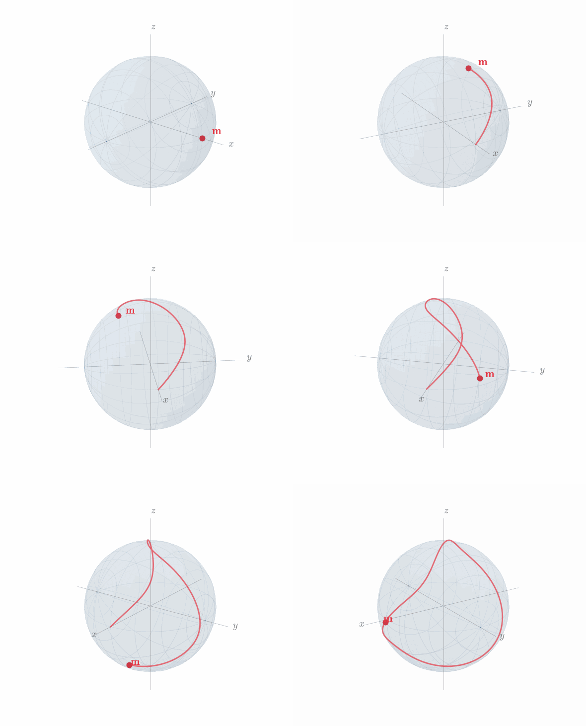
Figure 2 The reduced magnetization \(\mathbf{m}\) lives on the unit sphere \(\mathcal{S}^2\). The red marker represents the current orientation at a given spatial point.

Magnetization parametrizations

Because \(\mathbf{m}\) is constrained to \(\mathcal{S}^2\), any computational representation requires a choice of how to parametrize that manifold. Two classical families exist [Horley et al., 2009, Reichel et al., 2022].

Cartesian formulations store \(\mathbf{m}=(m_x,m_y,m_z)\in\mathbb{R}^3\) as three independent degrees of freedom. The constraint \(|\mathbf{m}|=1\) is not encoded in the parametrization and must be enforced externally at each step. Three approaches are common:

• Post-step renormalization rescales the solution after each accepted step, \(\mathbf{m}\leftarrow\mathbf{m}/|\mathbf{m}|\). The operation is inexpensive, but the renormalized point on \(\mathcal{S}^2\) is not the one a constrained integrator would reach, so a small directional error is introduced at each step. Over long, low-damping simulations this accumulates as artificial dissipation and phase drift [Abert, 2019, Kružík and Prohl, 2006].

• Penalty methods augment the energy density with a term \(\lambda(|\mathbf{m}|^2-1)^2\). Constraint satisfaction improves with increasing \(\lambda\), but large \(\lambda\) also stiffens the discrete system and degrades its conditioning.

• Lagrange multiplier methods impose the constraint weakly via an auxiliary scalar field, enforcing \(|\mathbf{m}|=1\) exactly at the continuous level. The price is a saddle-point system that requires inf-sup-stable discretization and specialized solvers.

Each approach carries a trade-off between accuracy, conditioning, and implementation complexity, which is why all three remain in use.

Intrinsic (parametric) formulations represent \(\mathbf{m}\) using only two coordinates on \(\mathcal{S}^2\), so that \(|\mathbf{m}|=1\) is satisfied by construction for any coordinate value, with no external enforcement required. The canonical example is the spherical-angle parametrization (Fig. Figure 3), which uses a polar angle \(\theta_0\in[0,\pi]\) measured from the \(z\)-axis and an azimuthal angle \(\theta_1\in[0,2\pi)\) in the equatorial plane:

(3)\[\mathbf{m}(\theta_0,\theta_1) = \bigl(\sin\theta_0\cos\theta_1,\; \sin\theta_0\sin\theta_1,\; \cos\theta_0\bigr)^\top.\]

Since \(|\mathbf{m}|^2=\sin^2\theta_0+\cos^2\theta_0=1\) identically, the unit-length constraint is encoded by the map itself with no post-processing. The induced metric tensor measures arc-lengths on \(\mathcal{S}^2\) in terms of coordinate increments, via \(|d\mathbf{m}|^2 = d\boldsymbol{\theta}^\top\mathcal{P}\,d\boldsymbol{\theta}\):

(4)\[\begin{split}\mathcal{P}(\boldsymbol{\theta}) = \begin{pmatrix} 1 & 0 \\ 0 & \sin^2\theta_0 \end{pmatrix}.\end{split}\]

The metric is diagonal but anisotropic: the polar direction has unit arc-length everywhere, while the azimuthal arc-length scales as \(\sin\theta_0\) and vanishes at the poles \(\theta_0=0\) and \(\theta_0=\pi\). There, all values of \(\theta_1\) map to the same physical point and the parametrization is no longer locally bijective. These poles correspond to \(\mathbf{m}\parallel\pm z\), states routinely visited during switching and precessional dynamics.

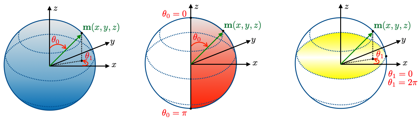
Figure 3 Spherical-angle parametrization on \(\mathcal{S}^2\). Left: the angles \(\theta_0\) (polar) and \(\theta_1\) (azimuthal). Centre: the singular poles \(\theta_0=0,\pi\) (red). Right: the azimuthal wrap-around \(\theta_1=0\equiv 2\pi\) (yellow).

The existence of such singular points is unavoidable for any intrinsic parametrization. Cartesian formulations are exempt because \(\mathbf{m}\) is treated as an unconstrained vector in \(\mathbb{R}^3\); the coordinate space is flat and globally non-singular. An intrinsic parametrization, by contrast, identifies \(\mathbf{m}\) with the image of a smooth map \(\boldsymbol{\phi}:\mathcal{U}\to\mathcal{S}^2\) from a coordinate domain \(\mathcal{U}\subset\mathbb{R}^2\). For this map to be a valid local chart, its derivative \(d\boldsymbol{\phi}\) — the two column vectors \(\partial\mathbf{m}/\partial\theta_0\) and \(\partial\mathbf{m}/\partial\theta_1\) — must span the tangent plane of \(\mathcal{S}^2\) at every point, i.e. they must constitute a smooth, non-vanishing tangent frame on \(\mathcal{S}^2\). The Hairy Ball Theorem [Eisenberg and Guy, 1979] asserts that no such frame can exist globally on \(\mathcal{S}^2\): the derivative of any single-chart parametrization must therefore lose rank at least at one point, producing a coordinate singularity. The choice of intrinsic parametrization therefore determines only where that singularity falls, not whether one exists.

The Landau–Lifshitz–Gilbert equation

The time evolution of \(\mathbf{m}\) is governed by the Landau–Lifshitz–Gilbert (LLG) equation [Gilbert, 2004, Landau and Lifshitz, 1935]:

(5)\[\frac{\partial\mathbf{M}}{\partial t} = -\gamma_0\mu_0\,\mathbf{M}\times\mathbf{H}_{\text{eff}} + \frac{\alpha}{M_\mathrm{s}}\,\mathbf{M}\times\frac{\partial\mathbf{M}}{\partial t},\]

where \(\gamma_0\) [rad/(T·s)] is the gyromagnetic ratio, \(\mu_0\) [T·m/A] the vacuum permeability, and \(\alpha\) [-] the dimensionless Gilbert damping parameter. The effective field \(\mathbf{H}_\text{eff}\) [A/m] is the variational derivative of the total micromagnetic energy with respect to \(\mathbf{m}\); its contributions (Zeeman, exchange, anisotropy, demagnetizing) are derived in Micromagnetic energy and Magnetostatics. The first term describes gyromagnetic precession: \(\mathbf{M}\) rotates around \(\mathbf{H}_\text{eff}\) at the Larmor frequency \(\omega_L=\gamma_0\mu_0|\mathbf{H}_\text{eff}|\) [rad/s], the angular precession rate of a magnetic moment in a field of magnitude \(|\mathbf{H}_\text{eff}|\). The second term is dissipative and drives \(\mathbf{M}\) towards alignment with \(\mathbf{H}_\text{eff}\) on a characteristic time scale \((\alpha\omega_L)^{-1}\).

Dividing by \(M_\mathrm{s}\) gives the normalized form in terms of \(\mathbf{m}\):

(6)\[\frac{\partial\mathbf{m}}{\partial t} = -\gamma_0\mu_0\,\mathbf{m}\times\mathbf{H}_{\text{eff}} + \alpha\,\mathbf{m}\times\frac{\partial\mathbf{m}}{\partial t}.\]

Both right-hand-side terms are cross products with \(\mathbf{m}\), so \(\partial_t\mathbf{m}\) is perpendicular to \(\mathbf{m}\) at all times:

(7)\[\mathbf{m}\cdot\frac{\partial\mathbf{m}}{\partial t}=0 \;\Longleftrightarrow\; \frac{d}{dt}|\mathbf{m}|^2=0.\]

The LLG equation therefore preserves \(|\mathbf{m}|=1\) exactly at the continuous level, consistent with the physical saturation constraint.

LLG in each parametrization

The choice of parametrization determines how well \(|\mathbf{m}|=1\) is preserved when the LLG equation is discretized in time.

Cartesian. The LLG equation (6) is integrated as a vector ODE in \(\mathbb{R}^3\). Standard implicit time-stepping schemes advance \(\mathbf{m}\) without enforcing the tangency condition (7) at the discrete level. As a result, \(|\mathbf{m}^{n+1}|\neq 1\) in general after any such step, even if \(|\mathbf{m}^n|=1\). The constraint must therefore be re-imposed at each step by one of the three external mechanisms described above, each carrying its own accuracy or conditioning cost.

Spherical-angle. Projecting (6) onto the tangent basis induced by (3) yields a \(2\times 2\) system in \((\theta_0,\theta_1)\), where \(\mathcal{L}(\boldsymbol{\theta})\) is the projected damping-precession matrix and \(\mathcal{F}(\boldsymbol{\theta})\) the corresponding right-hand-side vector [Dornisch et al., 2019, Yi and Xu, 2014]:

(8)\[\begin{split}\mathcal{L}(\boldsymbol{\theta})\,\dot{\boldsymbol{\theta}} = \mathcal{F}(\boldsymbol{\theta}), \qquad \mathcal{L}(\boldsymbol{\theta}) = \frac{M_\mathrm{s}}{\gamma_0} \begin{pmatrix} \alpha & -\sin\theta_0 \\ \sin\theta_0 & \alpha\sin^2\theta_0 \end{pmatrix}.\end{split}\]

Any update of \((\theta_0,\theta_1)\) maps back to \(\mathcal{S}^2\) via (3), so \(|\mathbf{m}|=1\) is satisfied exactly at every discrete step with no post-processing. However, the determinant \(\det\mathcal{L}=(1+\alpha^2)(M_\mathrm{s}/\gamma_0)^2\sin^2\theta_0\) inherits the metric singularity of (4): it vanishes at \(\theta_0=0\) and \(\theta_0=\pi\), rendering the system matrix rank-deficient at the poles and causing iterative solvers to stagnate or fail.

By the Hairy Ball Theorem, these singular points cannot be eliminated, only relocated. Stereographic formulation develops a parametrization that pushes the singularity to coordinate infinity, making it physically unreachable, and shows how Z-mag extends it to maintain well-conditioned coordinates everywhere on \(\mathcal{S}^2\).