Benchmarks

This chapter collects benchmark simulations used to evaluate the accuracy and robustness of the dual-chart stereographic solver. Each example is chosen to exercise a specific aspect of the formulation, and further cases will be added as the solver develops.

Precession and damping

The time evolution of a spatially uniform magnetization under a constant external field provides a direct test of gyromagnetic precession, damping-driven relaxation, and atlas adaptation in a well-controlled setting where no spatial gradients are present [Brach et al., 2026].

The simulation domain is a cubic box of edge length \(L = 1.0\,\ell_{\mathrm{ex}}\). The dynamics are driven solely by a uniform applied field aligned with \(+z\), \(\mathbf{H}_{\mathrm{ext}} = (0,0,1)\), with exchange, anisotropy, and magnetostatics absent. The initial magnetization is spatially uniform, set to the unit vector \(\mathbf{m}_0 = (0.92, -0.34, 0.18)\), which is misaligned with both the field and the chart poles. Simulations are performed for \(\alpha \in \{0.05, 0.1, 0.5, 1.0\}\) to cover the range from weakly damped precession to strongly damped relaxation. The two stereographic charts project from antipodal poles \(\mathbf{p}_A = (0,-1,0)\) and \(\mathbf{p}_B = (0,+1,0)\); since the precessional orbit encircles \(z\), the trajectory repeatedly crosses the equatorial band and visits the ill-conditioned neighborhood of each pole in turn, providing a stringent test of the atlas. The driver is test_dynamic_precession_damping.py.

Starting from the initial condition, the magnetization spirals smoothly toward the field-aligned equilibrium \(+z\). As \(\alpha\) increases, the number of revolutions about the field axis decreases and the spiral tightens: for \(\alpha = 0.05\) the trajectory completes many revolutions before converging, while for \(\alpha = 1.0\) it approaches equilibrium nearly radially with minimal angular displacement, consistent with the transition from underdamped precession to overdamped relaxation. The smooth and continuous character of the trajectories demonstrates that the dual-chart formulation provides a globally coherent representation throughout the evolution, with no artificial discontinuities arising from the chart structure.

The animations below show, on the left, the top-view projection of the magnetization trajectory on the unit sphere. On the right, the top row tracks the domain-averaged atlas weights \(\langle w_A \rangle\) and \(\langle w_B \rangle\) over time, while the bottom row shows the maximum stereographic radii \(|\mathbf{q}_A|\), \(|\mathbf{q}_B|\), and the effective radius \(|\mathbf{q}_{\mathrm{eff}}| = \min(|\mathbf{q}_A|,|\mathbf{q}_B|)\) (evaluated as a pointwise minimum and reported as a domain maximum). The atlas weights oscillate in counterphase as the magnetization precesses about the field axis, with decreasing frequency as equilibrium is approached. As the magnetization approaches the projection pole of one chart, the corresponding stereographic radius \(|\mathbf{q}|\) grows while the complementary chart remains well-conditioned; the effective radius \(|\mathbf{q}_{\mathrm{eff}}|\) remains below unity throughout all simulations, confirming that the atlas stays within the valid domain of the stereographic representation. Increasing \(\alpha\) reduces the time spent near the poles and the number of visible oscillations in the atlas diagnostics.

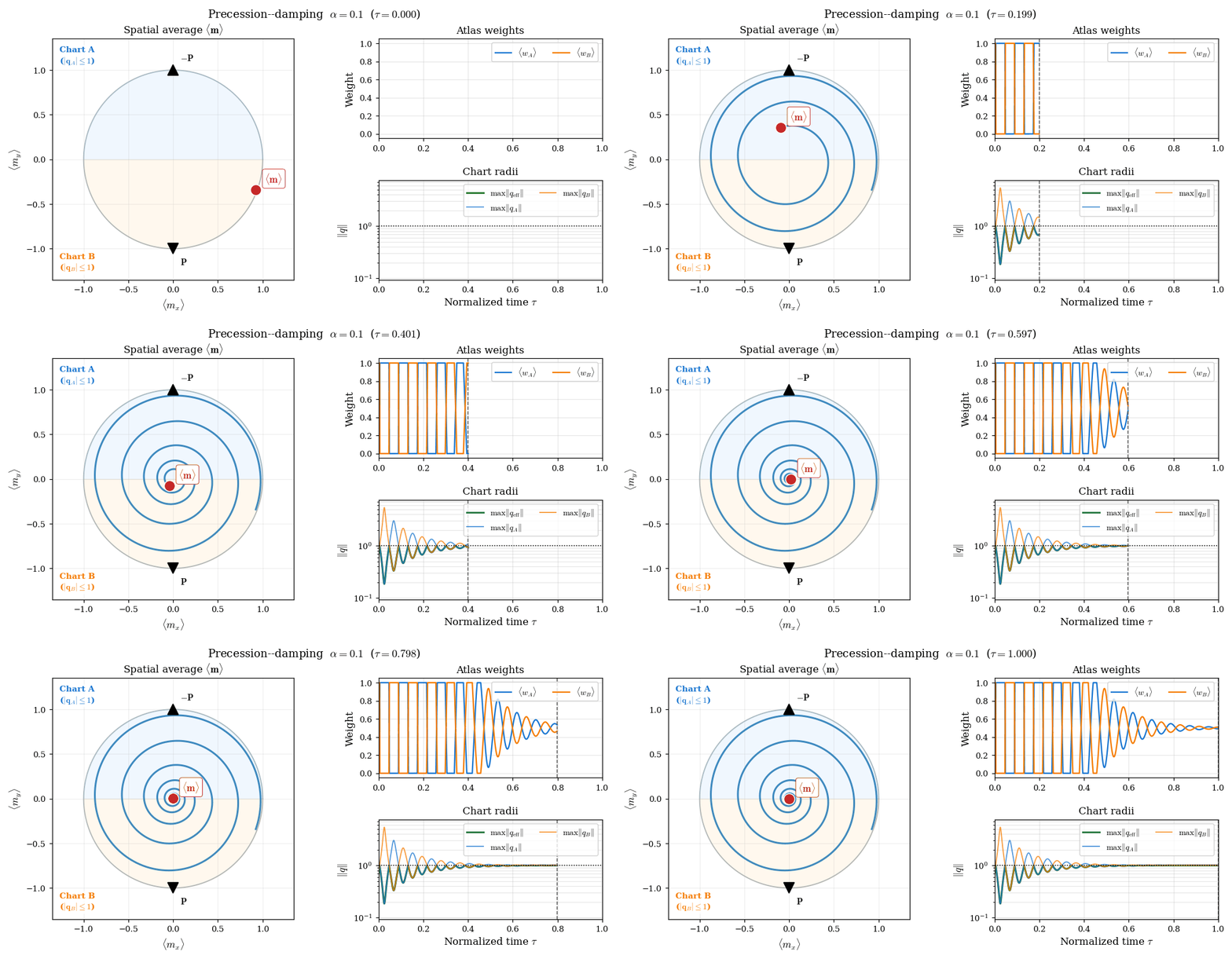
Figure 11 Precessional relaxation with \(\alpha = 0.1\). Left: top-view of the magnetization trajectory on the unit sphere spiraling toward \(+z\). Right (top): time evolution of the domain-averaged atlas weights \(\langle w_A \rangle\) (blue) and \(\langle w_B \rangle\) (orange), which alternate continuously as the precessing magnetization shifts the dominant hemisphere. Right (bottom): maximum stereographic radii \(|\mathbf{q}_A|\), \(|\mathbf{q}_B|\), and the effective radius \(|\mathbf{q}_{\mathrm{eff}}|\). With lighter damping the trajectory completes many revolutions, producing many oscillation cycles in the atlas diagnostics before convergence.

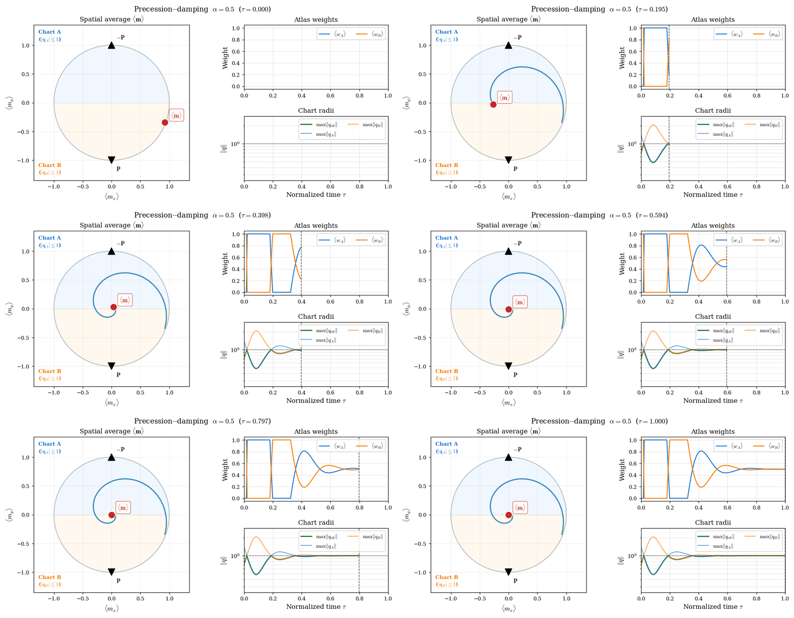
Figure 12 Same configuration with \(\alpha = 0.5\). Stronger damping shortens the spiral to two or three revolutions; the atlas weights complete a corresponding number of oscillation cycles and \(|\mathbf{q}_{\mathrm{eff}}|\) remains bounded before settling as the magnetization converges to the \(+z\) equilibrium.

\(\mu\)MAG Standard Problem 3

Standard Problem 3 (SP3) [Hertel and Kronmüller, 2002, NIST Center for Theoretical and Computational Materials Science, n.d.] is classically formulated as a static energy-minimization problem to determine the crossover cube size between the flower and vortex ground states of a cubic ferromagnet. Here the corresponding damped LLG relaxation dynamics are used instead, to assess whether the solver can robustly follow physically plausible pathways in a multistable system — a stringent test in the presence of strongly nonuniform magnetization configurations [Brach et al., 2026].

Simulations are performed for cubic magnets with edge lengths \(L = 8.0\)–\(9.0\,\ell_{\mathrm{ex}}\), spanning the known crossover region (typically reported near \(L \approx 8.4\)–\(8.6\,\ell_{\mathrm{ex}}\) depending on the numerical setup [Hertel and Kronmüller, 2002]). Material parameters follow the SP3 specification: \(M_s^* = A^* = K^* = 1\), uniaxial easy axis along \(z\), \(Q_1 = 0.1\), \(\alpha = 0.5\). The energy functional includes exchange, uniaxial anisotropy, and open-boundary magnetostatics (FEM–BEM). Chart poles are at \(\mathbf{p}_A = (0,-1,0)\) and \(\mathbf{p}_B = (0,+1,0)\). Each simulation runs for 6000 BDF2 time steps from two initial conditions described below. The driver is test_dynamic_std_prb3.py.

Flower initialization. The magnetization is seeded uniformly along the easy axis with a small random perturbation \(\boldsymbol{\eta}\) of amplitude \(\sigma\):

(184)\[\mathbf{m}_F(\mathbf{x}) = \mathcal{N}\!\left((0,\, 0,\, 1) + \boldsymbol{\eta}(\mathbf{x})\right), \qquad \boldsymbol{\eta} \sim \mathcal{N}(0,\sigma^2),\]

where \(\mathcal{N}(\cdot)\) denotes normalization to unit length. This seed places the system squarely in the axially-aligned flower basin.

Vortex initialization. The magnetization is seeded with a spatially varying orientation that rotates smoothly from \(+z\) to \(-z\) in the \(y\)–\(z\) plane as a function of the normalized coordinate \(\tilde{x} = x/L - 1/2 \in [-1/2,\,1/2]\) [Beg and Fangohr, n.d.]:

(185)\[\mathbf{m}_V(\mathbf{x}) = \mathcal{N}\!\left( \bigl(0,\; \sin\!\bigl(\tfrac{\pi}{2}\,\tilde{x}\bigr),\; \cos\!\bigl(\tfrac{\pi}{2}\,\tilde{x}\bigr)\bigr) + \boldsymbol{\eta}(\mathbf{x})\right),\]

with the same small noise \(\boldsymbol{\eta}\). At \(\tilde{x}=-1/2\) the seed points along \(-y\), at \(\tilde{x}=0\) it aligns with \(+z\), and at \(\tilde{x}=+1/2\) it points along \(+y\), providing a smooth vortex-like starting configuration that breaks the axial symmetry.

The figure below shows the energy relaxation curves, colored by the identified magnetic regime: flower (red), transition (orange), and vortex (blue). For flower initializations, the trajectories start in the flower-like metastable basin and pass through an intermediate transition regime before relaxing toward a vortex-like state — behavior consistent with the twisted-flower regime reported near the flower–vortex crossover [Hertel and Kronmüller, 2002]. For vortex initializations, the trajectories begin in a transitional configuration and relax toward the vortex-like equilibrium. The energy decreases monotonically at every accepted step, a direct consequence of the thermodynamic gate (Thermodynamic gate (phase E)). These trends are consistent with the established SP3 literature; the damped trajectories probe the energy landscape dynamically, so intermediate states and relaxation pathways may connect metastable configurations to a competing basin without coinciding with the static minimizer.

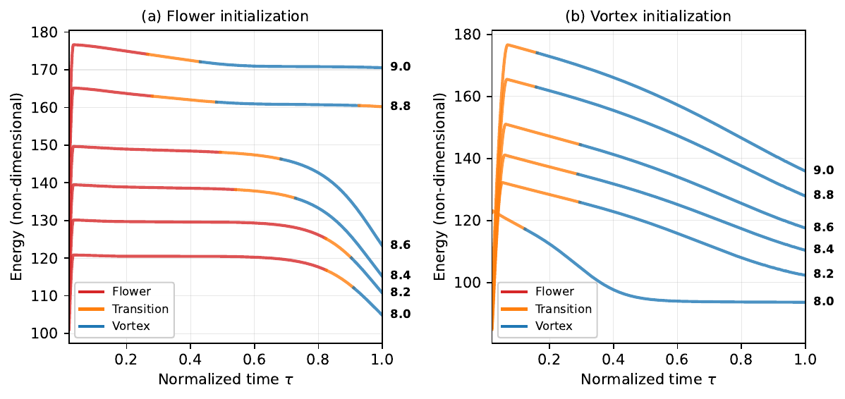
Figure 13 Energy relaxation during damped LLG dynamics for \(L = 8.0\)–\(9.0\,\ell_{\mathrm{ex}}\). Curves are colored by the identified magnetic regime: flower (red), transition (orange), vortex (blue). Left panel: flower initialization — trajectories leave the flower basin, pass through a transition regime, and approach a vortex-like state. Right panel: vortex initialization — trajectories relax monotonically toward the vortex equilibrium. Numbers indicate cube edge length in units of \(\ell_{\mathrm{ex}}\).

Checkpoint and restart chain

Long production runs are often split across cluster jobs. For that reason, Z-mag supports checkpointing and restart in both solver variants:

• demag — self-consistent magnetostatics via a hybrid FEM–BEM operator, including a demagnetizing potential phi.

• nodemag — the same adaptive implicit time integrator and atlas checkpointing, but without magnetostatics (so there is no phi and no BEM operator to rebuild).

The benchmark in test_dynamic_checkpoints.py focuses on the demag solver, because it additionally exercises the warm-start phi pathway and the need to rebuild the BEM operator after a restart.

The benchmark exercises this workflow as a chain of four consecutive restarts on MPI-parallel meshes, verifying that mesh tags, atlas fields, and BDF/controller history round-trip correctly while the thermodynamic gate remains active after each reload.

Problem setup. An elongated box (aspect ratio \(4{:}1\)) is magnetized along its long axis, with exchange, uniaxial anisotropy, and open-boundary magnetostatics. The run uses 50 accepted BDF2 steps with a checkpoint written every 10 steps. The protocol is:

1. Phase 1 — one continuous reference run, steps \(0\)–\(49\).

2. Restart 1 — load the step-10 checkpoint, run steps \(11\)–\(20\).

3. Restart 2 — load the step-20 checkpoint from Restart 1, run \(21\)–\(30\).

4. Restart 3 — load step 30, run \(31\)–\(40\).

5. Restart 4 — load step 40, run \(41\)–\(49\).

Each restart reads from the previous segment’s output directory, so the test validates repeated save/load cycles rather than a single resume from Phase 1.

What is checkpointed. A restart bundle combines three layers (see Checkpoints in Configuration reference):

• Distributed mesh — checkpoint_timestep_{step}.bp via adios4dolfinx (topology, geometry, cell/facet tags).

• Atlas + time integrator state — _qA.npz, _qB.npz, BDF history (_qA_prev, _qB_prev, …), chart metadata, and controller state (_time_state.npz: BDF order, dt caps, thermo EMAs, …).

• Demag potential — _phi.npz is present only in the demag variant, as a warm start for magnetostatics.

On restore, the restart segment reproduces the checkpointed fields to machine precision (\(\lesssim 10^{-10}\) relative error). That is the hard gate of the benchmark.

How restart works (in practice). A restart segment is always run by a fresh solver instance:

1. Build the solver and read the checkpoint header to recover the timestep step_start and the corresponding t_start/dt.

2. Rebuild the mesh and tags from the stored .bp file.

3. Assemble operators on the restart job’s MPI partition:

   • call the usual setup methods (set_mesh, set_materials, set_magnetostatics),

   • and, for model="demag", call set_BEMcpp after set_mesh.

4. Restore atlas and controller state with restore_checkpoint_atlas_state.

5. Initialize the restart solve with init_dynamic(first_run=False). For the demag solver this step is also where we reconcile magnetostatics: the stored phi is used only as a warm start; the code recomputes phi using the live BEM operator before seeding the thermodynamic baseline.

Why the mesh and BEM must be rebuilt. The key point is that read_checkpoint_mesh reconstructs the same global mesh, but not necessarily with the same MPI partition as the job that produced the checkpoint. adios4dolfinx redistributes cells across ranks, so the local DOF layout, ghost layers, and boundary-node ordering change.

For demagnetization, the BEM operator is assembled from the live partition’s exterior facet nodes. That means the restart job must rebuild the BEM matrix; the stored phi corresponds to the previous job’s BEM layout and can be inconsistent with the newly assembled operator.

Demag re-equilibration and thermo seeding. Restored chart fields q_A/q_B define the magnetization. In contrast, the demagnetizing potential phi depends on the magnetostatic operator (and thus on how the mesh is partitioned across MPI ranks).

If the restart kept the checkpointed phi without reconciliation, the first Newton iteration would effectively measure an operator swap instead of genuine LLG dissipation. In the checkpoint chain this would show up as a thermodynamic gate failure at the first post-restart step.

The demag solver therefore recomputes phi from the restored magnetization using the live BEM in init_dynamic. After that, the code seeds thermo_last_energy from the consistent (re-equilibrated) state. Checkpoint phi remains useful only as a warm start.

Energy in the continuous reference run. The logged total energy is the sum of the active terms written by compute_energy() (exchange, anisotropy, demagnetization). In this benchmark the magnetization starts nearly uniform along the easy axis, so exchange and anisotropy are initially small while demagnetization dominates the total. As the structure develops, exchange and anisotropy grow while demagnetization decreases. The total therefore falls at first, reaches a minimum near step \(31\), and then rises again because the gain in exchange/anisotropy temporarily outweighs the continued drop in demagnetization. This is visible in panel (b) of the figure below and is not a sign of a failed run: every accepted step in Phase 1 passed the thermodynamic gate.

What happens at a restart load. Immediately after restore_checkpoint_atlas_state the atlas fields match the checkpoint to machine precision (the hard gate of the test). The coloured traces in panel (a) then show how each restart segment evolves on its own MPI partition after adios4dolfinx redistribution. Because the FEM/BEM operators are reassembled on that partition, the trajectory can drift slightly above or below the Phase 1 reference even though the checkpoint itself is correct. Small upward or downward shifts at the first post-restart step are therefore normal and do not, by themselves, indicate corruption.

For the demag solver there is one additional effect that must be handled explicitly. The stored phi was computed with the BEM layout of the job that wrote the checkpoint. After remesh redistribution the live BEM operator changes, so keeping the old phi would make the first dynamical step look like a large artificial energy jump (often \(\mathcal{O}(0.1)\)–\(\mathcal{O}(1)\)). The code therefore recomputes phi from the restored magnetization in init_dynamic and only then seeds the thermodynamic baseline. That reconciliation removes the spurious jump; the remaining drift relative to Phase 1 is the partition-dependent numerical effect described above.

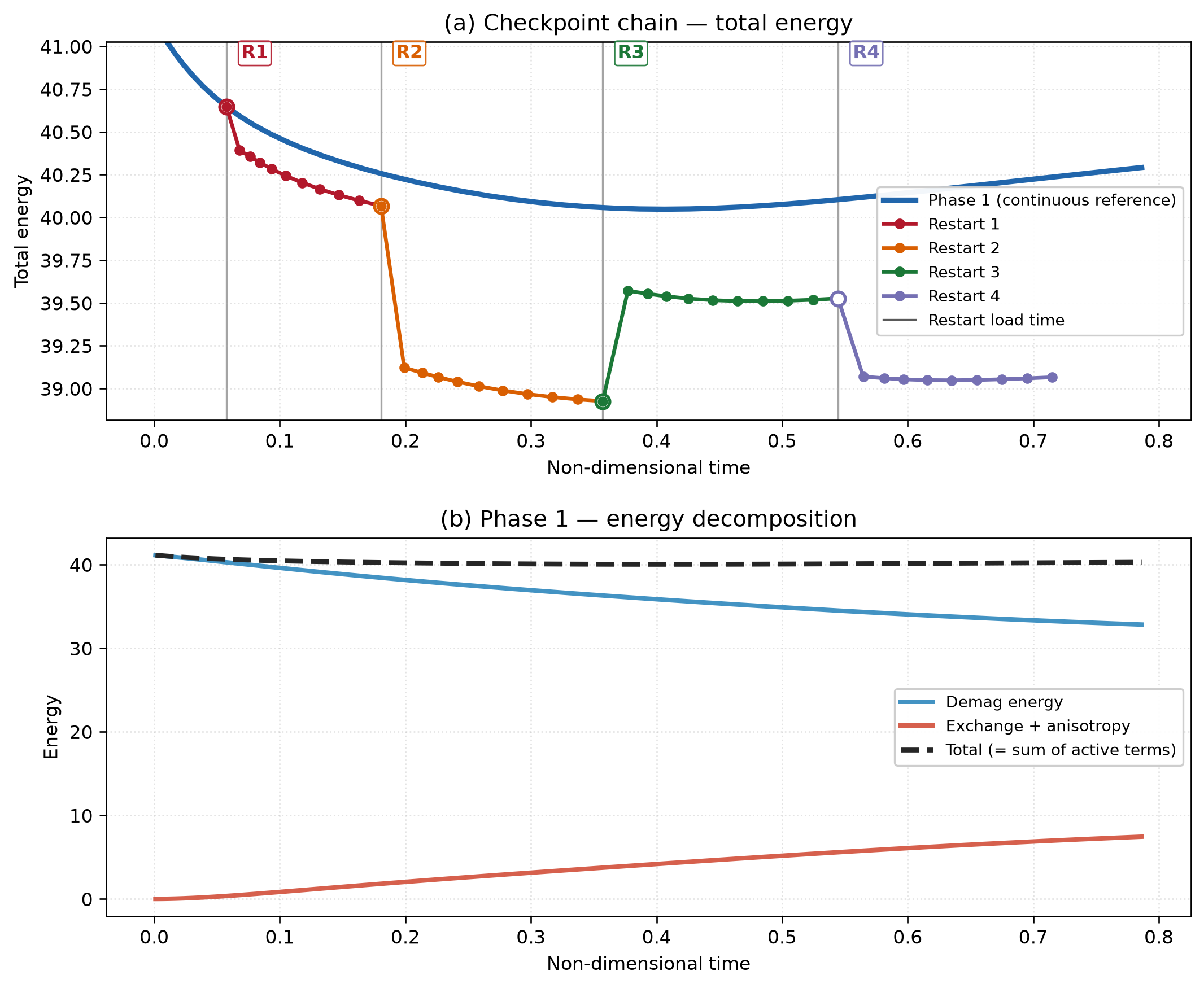
Figure 14 Checkpoint-chain benchmark (representative successful run). (a) Total energy: blue curve = continuous Phase 1 reference; coloured curves = restart segments loaded at the vertical grey lines (labels R1–R4). Segments agree at each load point, then drift apart because each restart uses a redistributed MPI partition. (b) Phase 1 energy decomposition: demagnetization falls while exchange + anisotropy rise; their sum explains the minimum and subsequent increase of the total in the continuous run.

Pass criteria. The driver reports PASS when

• cell/facet tag counts match on every restart, and

• restored atlas field norms match the ground truth to the required tolerance at every checkpoint in the chain.

Energy drift relative to Phase 1 is logged for inspection but does not fail the test. Reproduce with mpirun -n N python test_dynamic_checkpoints.py (see Installation).